Journal of Financial Planning: January 2016
Jerry A. Miccolis, CFP®, CFA, FCAS, MAAA, CERA, is a founding principal and the chief investment officer of Giralda Advisors (part of Montage Investments). He has more than 40 years of experience in the actuarial, risk management, and investment management fields, and is co-author of Asset Allocation For Dummies®.
Gladys Chow, CIMA®, is managing director and a portfolio manager of Giralda Advisors. She has spent more than two decades managing money for regulated investment companies, foundations, trusts, family partnerships, and institutional, corporate, and individual clients.
Rohith Eggidi, CFA, is an investment analyst at Giralda Advisors where he coordinates quantitative research and analysis, risk modeling projects, and development and maintenance of Giralda’s proprietary risk-managed investing solutions. He has prior experience in asset valuation and software engineering.
Executive Summary
- This paper outlines the “portfolio problem”—that most investors need a sizeable allocation to so-called “risk assets” such as equities in their portfolio, but large drawdowns in the market value of these assets are quite frequent. Other asset classes whose key purpose is to buffer the risk of the equity asset class have become problematic and often detrimental to portfolio performance.
- “Risk-managed investing” (RMI) attempts to address the portfolio problem directly by going beyond asset allocation to explicitly mitigate equity risk within the equity investment itself by dampening equity volatility and/or limiting its downside potential.
- This paper empirically quantifies the benefits of downside protection, thereby gauging its cost-effectiveness. Modestly effective downside protection is shown to support a cost, in terms of performance drag in rising markets, of several hundred basis points of return per year.
- The quantitative techniques in this paper can be used by investment professionals to objectively gauge the efficacy of proposed RMI solutions in the marketplace, several of which are briefly outlined.
In the wake of the financial crisis and ensuing equity market collapse of 2008–2009, there has been a proliferation of strategies and products that attempt to dampen the volatility—and in some cases explicitly limit the downside risk—of equities. Each of these approaches has a cost, whether implicit or explicit, and some strategies are more cost efficient than others.
The “Portfolio Problem” and a Potential Solution
Let us put this topic into perspective by framing what we believe is the most significant financial planning issue facing clients over the next several decades—what we call the “portfolio problem.” This problem is unique in the last 30 years, therefore unique in the careers of most financial planners. To meet their long-range financial goals, virtually all investors need a sizeable allocation to “risk assets,” such as equities, in their portfolio; however, large drawdowns in the market value of these assets are quite frequent. The S&P 500 Total Return Index, for example, suffered non-overlapping drawdowns of –10 percent or worse 29 times from 1935 through 2013, a frequency of once every 2.7 years on average.
Other asset classes found in many client portfolios, such as fixed income and liquid alternatives, whose key purpose is to buffer the risk of the equity asset class, have become problematic. It is, mathematically, highly improbable for traditional fixed income investments to achieve, over the next decade or so, the kind of total returns they have enjoyed over the last 30 years, a period during which interest rates have steadily fallen from their substantial heights. Attempts to boost the total return expected from traditional fixed income investments in the current environment by moving into lower-credit-quality bonds, for example, tends to increase the correlation with equities, thus compromising a key mandate of fixed income investments. This fixed income dilemma is the primary reason the portfolio problem is unique in the last three decades.
Liquid alternatives have become similarly challenged. For the most part, their returns have turned mediocre as the space has become more crowded, and they have shown increasing levels of correlation with equities. Moreover, clients may be impatient with diversified portfolios that have consistently underperformed headline passive indexes, such as the S&P 500 over the past several years.
A possible solution to the portfolio problem is provided by investments that attempt to manage equity risk directly within the equity investment itself. We label such attempts as “risk-managed investing” (RMI).
The following summary outlines the various categories of products and solutions currently available, covering both volatility dampening and downside protection elements of RMI:
- Strategies that employ tactical rotation out of equities and into other asset classes, and vice versa, based on fundamental analyses regarding the state of the economy and the capital markets.
- “Low volatility” or “minimum volatility” or “risk control” funds that attempt to deliver equity exposure with less volatility via stock screening and/or targeted volatility approaches.
- Quantitative momentum-based strategies that employ moving average or other algorithms to signal movements into and out of asset classes and/or sectors within asset classes.
- Tail risk hedging overlays that employ equity options (such as puts, put spreads, collars, etc.) and/or “investments in volatility” (such as variance swaps and volatility futures).
- Various combinations of the above.
Each of these RMI categories, and each of the available products within the categories, may be appropriate in the proper situation. It is not our objective here to judge their relative worth in the absence of specific client circumstances. Each may warrant investigation. A key objective of this paper is to provide a rigorous empirical framework within which to compare the efficacy of various candidate approaches to assist financial planners in such an investigation. This new framework is necessitated by the fact that the more standard measures of assessment—such as standard deviation, alpha, beta, maximum drawdown, upside/downside capture—tend to be collectively incomplete with regard to RMI.
One notable feature of RMI is its potential to raise the efficient frontier of possible portfolios and thereby allow the adviser to “re-risk” the client’s portfolio advantageously.
RMI would appear to solve the portfolio problem, but there is a catch. RMI vehicles typically have a cost, either explicit (fees, expenses, option premiums) or implicit (sacrifice of equity upside potential) that manifests itself to the investor as a performance drag (relative to broad equity indexes) in up-trending markets. Over full market cycles, this cost can outweigh the risk management benefits. For RMI to be truly worthwhile, then, its cost needs to be sufficiently low. It is the main objective of this paper to quantify how low that cost needs to be.
Preliminary Observations
Although this paper focuses on the downside protection element of RMI, it is important to note that RMI approaches that succeed in providing downside protection also, by definition, succeed in dampening volatility. Volatility dampening itself has a number of demonstrable benefits, both qualitative and quantitative.
On the qualitative side, some investors may place high emotional value on predictability and peace of mind, perhaps above other considerations. This, by itself, may be sufficient reason for these investors to consider equity investing strategies that purport to control volatility. Moreover, many investors fear short-term equity risk to such a degree that they hold a smaller equity allocation than their financial planning projections indicate that they should. In other words, they allow this fear to deny them access to a properly balanced portfolio designed around their specific financial goals and circumstances. Allowing these individuals to hold the appropriate amount of equities by directly mitigating their short-term volatility through RMI provides a qualitative benefit that could be considerable.
Volatility dampening provides two primary quantitative benefits. The first is the reduction of “volatility drag,” or the erosion in multi-period compound returns caused when the returns of each period vary considerably from one another. It is easy to construct examples of how a steady 8 percent annual return, for example, can result in greater ending wealth than a fairly erratic return stream that averages 9 percent. Volatility drag increases with volatility, thus RMI’s volatility dampening can add value by increasing compound returns in a very straightforward and quantifiable way.
The second benefit is mitigation of sequence of returns risk or, more simply, sequence risk, which occurs when the specific sequence of periodic returns is such that it impairs the financial condition of the investor, relative to a more favorable sequence of the same periodic returns. This can happen when there are substantial flows into or out of the investment account, such as when a severe market downturn occurs immediately before the investor needs to make a significant portfolio withdrawal. The more stable the return stream, the less the sequence risk. While no practical RMI technique can totally eliminate return volatility, every step in that direction adds value from a sequence risk perspective.
Investment approaches that provide downside protection can deliver additional advantages. The remainder of this paper is an examination of the historical record to attempt to quantify these additional benefits. It is important to note that the benefits measured in the following analysis do not explicitly include the qualitative and quantitative advantages thus far described and, therefore, can be considered a conservative estimate of the total benefit.
Return Asymmetry
It is a well-known, but perhaps underappreciated, fact that positive and negative returns are asymmetric; that is, every –1 percent decline requires greater than a +1 percent recovery to get the investor back to breakeven. The larger the percentage, the more pronounced the asymmetry. This is generalized in Table 1.
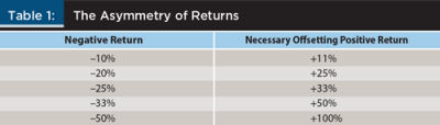
The immediate takeaway from Table 1 is that in terms of percentage returns, avoiding a loss is the economic equivalent of capturing a gain of greater magnitude. This has major ramifications. To help quantify these ramifications, the following discussion reviews some relevant history.
A Look at Equity Market History
The equity markets are characterized by recurring periods of decline and recovery. The long-term (1936–2013) average annual return of the S&P 500 Total Return Stock Index1 was approximately 11 percent. The overall upward tendency in the markets has been interrupted by periods of substantial decline. As Figure 1 shows, over the 78-year period from the end of 1935 (when total return data on the S&P 500 first became available) through the end of 2013, there were 29 separate, non-overlapping episodes of market declines that were each worse than –10 percent.2 This equates to a frequency of once every 2.7 years (32 months), on average.
Data for Figure 1 are based on the following: date of the local peak of the index; index value at that peak; date of the subsequent local trough (after the –10 percent-or-worse decline); index value at that trough; length of drawdown (peak-to-trough) period; percentage drawdown; date of recovery (when the index re-achieves its prior peak); length of that recovery period; recovery percentage; date of the next local peak (just prior to beginning its next –10 percent-or-worse decline); index value at that peak; length of cyclical bull (trough-to-peak) period; and, finally, the percentage increase during the bull period.
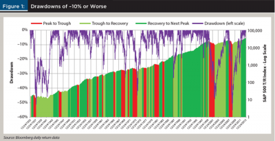
The recovery period is a subset of the bull period (in terms of the graph, the recovery period is shaded light green, and the bull period is the combined light and dark green shaded sections). Note that the final bull period was not complete as of December 31, 2013.
The average decline during those peak-to-trough periods (the red regions of the graph) has been approximately –21 percent. The average length of those periods has been about seven months. Representatively, the subsequent trough-to-peak upswing (the combined light and dark green regions of the graph) has been roughly 68 percent cumulatively. These periods have lasted about 25 months before the next –10 percent-or-worse downswing began. Assuming a $100 initial investment in this market at the beginning of a representative downdraft, it would decline to $79 over the first seven months, then rebound to $132.72 over the next 25 months. These figures are consistent with the long-term annual average market return of approximately 11 percent (this is how the representative trough-to-peak upswing of 68 percent was derived).
Examining Downside Protection
Typically, when downside protection is mentioned, most investors think in terms of put options. A 10 percent out-of-the-money put on the S&P 500 Total Return Stock Index, for example, will provide, for any loss in the index that exceeds the threshold defined by the put’s strike price (90 percent of the value of the index at the time the put was purchased in this case) 100 percent protection against the excess loss beyond that threshold. However, such a put will not provide 100 percent protection against the episodes previously defined, because those episodes were defined in terms of drawdown from peak to trough.
For a put to provide true peak-to-trough protection, the strike price would need to be continually adjusted upward whenever the index reached a new peak, and that is typically quite often. Furthermore, any time that the put was exercised (and, to provide true 100 percent protection, it would need to be exercised immediately on the day that the index falls –10 percent from its prior peak), it would need to be replaced seamlessly with another put, but this put would need to be at-the-money. The chance of needing to exercise that put in the near future is almost a certainty, at which point it would need to be replaced with another at-the-money put, and so on. This method of protection via puts, aside from being extremely expensive, is not feasible as a practical matter.3 To be realistic, we examined forms of downside protection that provide less than 100 percent impact on a drawdown (peak-to-trough) basis.
To formalize the analysis, we defined the following metrics for each RMI strategy under consideration:
- At what point is downside protection provided? (How deep a peak-to-trough drawdown does the strategy respond to?) We call this metric D.
- To what degree is protection provided? (What percentage of damage is mitigated once D is breached?) We call this metric p.
- How much does it cost? (What is the performance drag when protection isn’t needed?) We call this metric C.
It can be seen that the economic value of protection is a function of the first two metrics, i.e.:
EV = f(D,p)
The cost of the RMI strategy can be considered “tolerable” if:
C < f(D,p)
Equivalently, this tolerable cost can be denoted as CT, where:
CT(D,p) = f(D,p).
What follows is an empirical derivation of this critical function CT.
Quantifying the Value of Downside Protection
What is the impact if downside protection were applied to the episodes identified from the return history of the S&P 500 Total Return Stock Index? These episodes, which reflect drawdowns of –10 percent or worse, are therefore relevant for assessing RMI strategies whose drawdown threshold metric, D, is –10 percent.
Recall that the average peak-to-trough decline during those episodes has been approximately –21 percent. The subsequent trough-to-peak upswing has been roughly 68 percent. Let us examine the RMI strategy that provides 50 percent downside protection against a decline threshold of –10 percent; that is, one where the D and p metrics are –10 percent and 50 percent, respectively. Such a strategy succeeds in modestly reducing the decline on an initial $100 investment from –21 percent to –15.5 percent (by half the excess decline beyond –10 percent), net of the cost of the strategy. In this case, if the subsequent 68 percent upturn is unimpeded, the result after the full 32-month cycle would be $141.96, which is a much better result than the $132.72 that the market would deliver in the absence of RMI. This result would imply a long-term average annual return of 14 percent instead of 11 percent.
It is unrealistic to assume that an RMI strategy could successfully reduce the downside, however modestly, and not have some cost, our metric C. It is useful to think of C in terms of a performance drag on the upside, as that is the way the investor would experience it. The simple 32-month model provides a way to estimate how large C could be without negating the benefit of the downside protection. Specifically, if the seven-month decline on the $100 investment is –15.5 percent (net of the cost of the strategy) instead of –21 percent, then the subsequent 25-month bull market run need be only 57 percent cumulatively, instead of 68 percent to achieve the “breakeven” value of $132.72.
What does this mean in terms of the annual tolerable cost, CT? The annualized version of the 68 percent, 25-month return is 28.3 percent, while the annualized version of the 57 percent, 25-month return is 24.2 percent. The difference is 410 basis points. So, here is the result: if history is a guide, an RMI strategy whose downside protection reduces only large declines in the equity markets (those worse than –10 percent), and reduces them only modestly (specifically, by half their excess beyond –10 percent) adds measurable value as long as its cost (i.e., its performance drag during bull markets) does not exceed 410 basis points per year. In other words: CT(–10 percent, 50 percent) = 410 bps.
This kind of RMI strategy is realistically achievable.
To give some additional context to the previous result, consider an RMI strategy that reduces the impact of portfolio downturns by 50 percent of the excess downturn beyond –10 percent whose cost amounts to an annual performance drag C during bull markets of 250 basis points, which is 160 basis points better than the 410 basis point CT derived previously. Consider now its impact over the investment horizon of a newly married couple just leaving college. The probability of at least one spouse living into his or her late 90s is sizeable enough that prudent financial planning should consider a remaining investment horizon of 75 to 80 years for this couple. If these years are a reasonable facsimile of the 78 years of history we have just examined, every dollar invested by the newlyweds in the RMI portfolio will have grown to more than twice as much as it would have in a non-RMI portfolio over that
horizon (using Excel notation: (((1–0.155)*(1.283–0.025) ^ (25/12))/((1–0.21)*(1.283) ^ (25/12))) ^ 29 = 2.14).
This example shows that even if the couple was very risk tolerant and did not pursue RMI for strictly defensive purposes, the value of cost effective RMI over several market cycles can be substantial from a pure return standpoint.
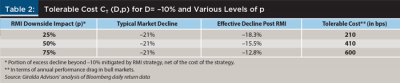
Generalizing the Results
Rounding out the analysis, Table 2 shows the tolerable cost CT of other theoretical RMI strategies that have varying levels of impact on mitigating downturns. The same 32-month model from the previous section was used to generate Table 2. For example, an RMI strategy whose downside protection reduces declines worse than –10 percent by three-quarters of their excess beyond –10 percent adds measurable value as long as its cost does not exceed 600 basis points per year. That is, CT(–10 percent, 75 percent) = 600 bps. Similarly, we find that CT(–10 percent, 25 percent) = 210 bps.
It can be dangerous to apply an operation to an average input and expect the result to be representative of what a financial planner is really after, which is the average result obtained by applying the operation to each input separately. This has been referred to as the “flaw of averages” (Savage 2012). To address this issue, we also took a more detailed approach as shown in Table 3.
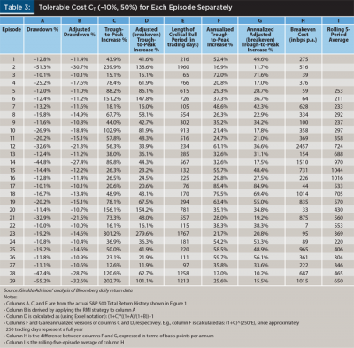
In this more detailed analysis, we applied the same RMI strategies as noted previously to each of the 29 peak-to-trough-to-peak cycles in the S&P 500 Total Return Index history, each of which encompassed a variety of investment horizons. This approach leads to a range of tolerable costs for each RMI strategy. For example, an episode with a shallow decline below –10 percent and an exceptionally long subsequent bull market period would lead to a tolerable cost that would be at the low end of the range.
The calculations are spelled out in the notes on Table 3. Column H of the table shows the tolerable performance drag for each episode in isolation. Because the length of each episode’s full cycle is generally much shorter than a typical investor’s investment horizon, we calculated successive rolling five episode averages of column H in column I to obtain results more in line with realistic investment horizons. From column I, we derived the 25th and 75th percentiles. These are shown in the middle row of Table 4. The percentiles shown in the top and bottom rows of Table 4 were derived similarly.
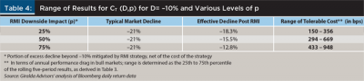
The results shown in Table 4 are consistent with those of Table 2. In our judgment, therefore, the quantification in Table 2 is robust and can be relied upon. That said, it is important to remember that there were, in fact, outlier episodes with results beyond these ranges. There is no guarantee that the next episode will not be another outlier.
It is possible to generalize the results further still. Other decline thresholds D can be chosen and the quantification would proceed precisely along the lines we have outlined above. Table 5 shows the results for drawdown thresholds of –5 percent and –15 percent, in addition to the –10 percent threshold already discussed.
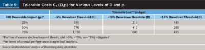
For example, using data in Table 5, an RMI strategy whose downside protection reduces declines worse than –5 percent by three quarters of their excess beyond –5 percent adds measurable value, as long as its cost—its performance drag during bull markets—does not exceed 1,130 basis points per year. That is, CT(–5 percent, 75 percent) = 1,130 bps.
Some RMI techniques, however, may not lend themselves to measurement along the lines thus far described. For example, some may follow the same general risk management approach, such as protection beyond a threshold, but their impact may be more or less precise, or certain, than implied above. Those situations can easily be modeled by applying the strategy directly to the relevant historical episodes and deriving the tolerable performance drag during the succeeding or preceding bull market period. Whichever way a particular RMI strategy may deliver its mitigating effect, the quantification approach outlined here should provide a useful roadmap to measuring the economic value of that effect.
The tolerable cost estimates, CT, derived through this analysis are conservative. One reason for this is that these estimates focus solely on quantifying the benefits of downside protection, consistent with the focus of this section of the paper. Even RMI strategies that are aimed solely at downside protection serve to provide a measure of volatility dampening as well. In this section, we have not given any consideration to those additional beneficial effects, such as mitigation of sequence risk, nor have we reflected any qualitative benefits, such as containment of fear, peace of mind, and quality of life. Considering these benefits would make the tolerable costs of RMI higher still. In particular, helping investors find the fortitude to stay true to their long-term allocation to risk assets during turbulent times may deliver the biggest benefit of all, and therefore support a tolerable cost well beyond those we have attempted to directly quantify here.
Another Dimension of Value
From a total portfolio perspective, there is an important dimension of value that has not yet been considered. The derivation of CT has concentrated solely on cumulative return. But RMI strategies, by virtue of their risk-dampening properties, can also mitigate portfolio risk and thereby elevate the efficient frontier.
A simple illustration of this phenomenon is shown in Figure 2, where we plot, in blue, the frontier of a two asset stock/bond portfolio, using the S&P 500 Total Return Index and the BarCap Aggregate Bond Total Return Index to represent the two assets. Twenty years of daily return data (December 30, 1994 to December 31, 2014) was used, and rebalancing was ignored for simplicity. The 60/40 point identified on the blue frontier signifies a portfolio of 60 percent stocks and 40 percent bonds.
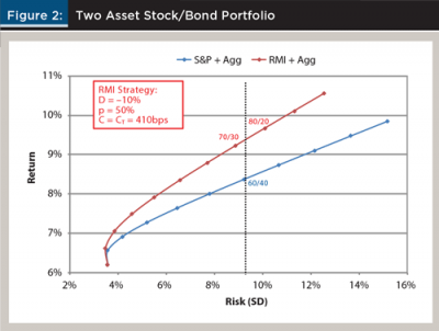
On the same Figure, we plot, in red, the efficient frontier obtained by substituting for the S&P 500 an RMI investment with the metrics D = –10 percent, p = 50 percent, and C = CT(–10 percent, 50 percent) = 410 basis points; that is, we used an RMI strategy which had a cost at the breakeven level as we have thus far defined it. The red, RMI-enhanced frontier is seen to be elevated above the blue.4
Although this is intended as a simplified illustration, it is important to note that RMI’s ability to elevate the efficient frontier is to be expected. This allows financial planners the opportunity to “re-risk” their clients’ portfolios. In the example, a planner can construct a portfolio that is risk-equivalent to a traditional 60/40 portfolio but, by introducing RMI, adjust the portfolio to approximately 75/25 and enjoy higher expected returns. Recall that this example used an RMI strategy with a “breakeven” cost (C = CT); a more cost-effective RMI strategy would elevate the frontier higher still, and allow greater re-risking benefits, moving the risk equivalent RMI portfolio toward, and perhaps beyond, 80/20.
The implications of this finding are potentially paradigm shifting, leading to fundamental changes in the way portfolios are constructed. Replacing a sizable portion of traditional equities within the portfolio with cost-effective RMI counterparts can reduce an investor’s need to rely on non-equity asset classes to manage downside risk. The investor can therefore lower the allocation to non-equity assets and correspondingly raise the allocation to (risk-managed) equities. A 75/25 or 80/20 portfolio could actually be safer in down markets and better performing in up markets than a traditional 60/40 portfolio is likely to be, particularly given the challenges outlined earlier for non-equity asset classes.
The intent in this paper was to focus on RMI conceptually and assess its potential impact on investors, without discussing the merits of any individual product or solution available in the marketplace. The approach used here contributes to the literature by helping to establish a solid foundation for the fair evaluation of products and solutions that have been, and like likely will be, brought to market in this growing area.
Endnotes
- Total return indexes include dividends, which are then assumed to be reinvested. Quotations of the S&P 500 in the popular press often reflect only price returns, which exclude dividends. Total return indexes are appropriate for analyses such as those in this paper.
- In defining each non-overlapping episode, we first required the index to reach its prior peak. For example, the drawdown of –17 percent in July/August 2011 was not counted as a non-overlapping episode because the index had not yet reached its prior peak. If such overlapping episodes had been counted, there would have been more than the 29 examined, and the benefits quantified in this paper would have been greater.
- There exist, in concept, instruments such as “Russian options” and “exotic look-back options” that are constructed along these lines but, to our knowledge, viable liquid markets for such instruments do not exist. In contrast, RMI strategies that deliver protection of less than 100 percent are feasible. Examples include those described in Miccolis and Goodman 2012a; Miccolis and Goodman 2012b; and Miccolis and Chow 2015.
- Two factors elevate the frontier in Figure 2. One is the reduction in portfolio standard deviation. The other is the fact that this 20-year period happens to support a higher CT than the one derived earlier using the 78-year (1935 to 2013) period. The BarCap Aggregate Total Return Index does not exist as far back as the S&P 500, so corresponding 78-year periods could not be used for this exercise. Thus, the derived RMI returns are higher than the corresponding S&P 500 returns, and not approximately equal, as one would expect when setting the cost, C, at the breakeven level, CT. Note that the first factor—the reduction in portfolio standard deviation, which moves the efficient frontier leftward—is the only factor necessary to elevate the frontier and the one that drives the opportunity to “re-risk” the portfolio.
References
Miccolis, Jerry, and Marina Goodman. 2012a. “Dynamic Asset Allocation: Using Momentum to Enhance Portfolio Risk Management.” Journal of Financial Planning 25 (2): 33–42.
Miccolis, Jerry, and Marina Goodman. 2012b. “Integrated Tail Risk Hedging: The Last Line of Defense in Investment Risk Management.” Journal of Financial Planning 25 (6): 44–53.
Miccolis, Jerry, and Gladys Chow. 2015. “Tail Risk Hedging: State of the Market.” Journal of Financial Planning 28 (9): 35–36.
Savage, Sam. 2012. The Flaw of Averages: Why We Underestimate Risk in the Face of Uncertainty. Hoboken, NJ: Wiley.
Citation
Miccolis, Jerry, Gladys Chow, and Rohith Eggidi. 2015. “Quantifying the Value of Downside Protection.” Journal of Financial Planning 29 (1): 50–57.