Journal of Financial Planning: January 2012
Executive Summary
- The market crash in the fall of 2008 exposed many problems with the oversimplifying assumptions often used in implementing the modern portfolio theory (MPT) framework.
- We describe more sophisticated methods of estimating the three principal assumptions used in MPT—returns, risk, and relationships. We also discuss ways of improving the optimization process itself.
- Key improvements include:
- Returns—parse market data into “quiet” and “turbulent” regimes to better understand how assets perform under different environments.
- Risk—add shortfall probability and conditional value at risk to your arsenal of risk measures.
- Relationships—use copula dependency functions instead of one-dimensional correlation statistics to fully capture how assets behave relative to each other in different markets; this is a powerful tool to identify the degree to which the portfolio is vulnerable to contagion.
- Optimization process—provide the capability to incorporate the above enhanced inputs, allow for non-normal distributions of returns, and recognize that an investment horizon is not a single uninterrupted period. This allows the optimizer to reflect how volatility erodes returns and show the beneficial effects of rebalancing.
- This is all just one step toward the goal of bringing investment risk management into the next generation for financial planners.
Jerry A. Miccolis, CFA, CFP®, FCAS, is a principal and the chief investment officer at Brinton Eaton, a wealth management firm in Madison, New Jersey, as well as a portfolio manager for The Giralda Fund. He co-authored Asset Allocation For Dummies® (Wiley 2009) and numerous works on enterprise risk management.
Marina Goodman, CFP®, is an investment strategist at Brinton Eaton and a portfolio manager for The Giralda Fund. She has been working to bridge the gap between research and practice in improving the portfolio optimization process, and has written numerous articles on the subject.
One Monday morning in mid-September 2008, financial planners suddenly found themselves in a new environment—one that was unprecedented in their lifetimes, and in many ways unprecedented in history. That day, and in the days that followed, it became very clear that the practice of portfolio management, which had been steadily evolving and improving over many years, needed to take a quantum leap forward. On that day, it’s fair to say, many of us in the financial planning industry found ourselves unprepared.
The events of late 2008 and early 2009 served as a particularly painful reminder that precipitous market declines can and do occur with far-reaching implications. Investors on all points of the asset allocation spectrum saw the values of their portfolios evaporate. Virtually every asset class—and there were more of them to invest in than ever before—fell victim to contagion, rendering portfolio diversification temporarily impotent. Against this grim backdrop toiled our industry—we who have a duty to our clients to seek out the best risk management solutions possible to help clients protect their assets against the ravages of the markets.
It became apparent that a far more comprehensive view of risk was required, one that took portfolio diversification—and, more generally, investment risk management—to a whole new level of sophistication. Although wealth destruction the likes of three years ago may never recur, our clients are not apt to be so forgiving should we again be unprepared if it does. In a very real sense, we are in a race against time. The “flash crash” of May 2010 and the more recent volatility of late 2011 make this need for urgency clear.
In this article, we describe the first component of our response to that challenge. We propose some key improvements in the conceptual approach to portfolio risk management and identify the tools needed to implement these enhancements. The improvements we suggest are quite achievable. In our firm, we have already implemented, or are in the process of implementing, all of them.
MPT Itself Was Not the Culprit
Why was our industry not successful in mitigating the effects of the market crash of 2008 for its clients? One key reason was a naïve understanding of diversification. Although advisers believed their clients were well diversified, during those fateful six months in late 2008 and early 2009, diversification did not work, as virtually all asset classes and sectors declined in unison.
The importance of diversification in building a solid portfolio was clearly articulated in Harry Markowitz’s modern portfolio theory (MPT). In his breakthrough paper published in 1952, he stated that the three key inputs in determining an optimal allocation among assets are the assets’ forecasted returns, projected risks, and expected interrelationships. After making some simplifying assumptions, he derived a mathematical formula for the optimal asset allocation given those three inputs.
One of the things the investment community adopted widely was the manner in which Markowitz measured return, risk, and relationships. Historical average returns were used as estimates of forecasted returns, historical standard deviations as estimates of projected risk, and correlation coefficients as estimates of expected interrelationships. Furthermore, Markowitz assumed that returns followed a normal (Gaussian) probability distribution. These simplifying assumptions were necessary in 1952 to make the math solvable by hand. However, Markowitz himself stated that these were just necessary simplifications at the time and not prescriptive values or approaches.
The drawbacks of the above simplifications of MPT are well documented.1 Historical returns are not good estimates of future returns, and returns are not normally distributed but have distributions that show far higher probability of large losses. Standard deviation measures dispersion around the average returns, not investors’ risk of losing money or failing to meet their objectives, which are closer to the way investors actually view their risk. Correlation coefficients assume that the varied and complex and dynamic relationships among different assets can be summarized by a single number—a simplification that is unnecessarily unrealistic. However, these simplifications stuck and are still being widely used.
If you put the results of these simplified assumptions together, you start to see the fault lines in what was thought of as proper diversification. Assets had distributions of returns with far greater chances of loss than implied by a normal distribution. The true amount of risk even in historical returns was hidden by the standard deviation, which did not distinguish between deviations above the mean (very positive returns) and deviations below the mean (very negative returns). Finally—and this was the hammer that smashed what many thought of as diversification—using one number as a measure of a relationship doesn’t allow the investment manager to distinguish between normal markets and stressed markets in modeling asset interrelationships. An investment manager may have thought a portfolio was diversified because it held assets with fairly low correlation to each other, when in fact these assets were only uncorrelated in relatively unstressed markets. They became most correlated when you most needed them not to be.
Many articles have been written heralding the death of MPT. MPT was not the culprit in 2008, and its conceptual framework is just as relevant as ever. That period, however, did highlight the danger of continuing to make 60-year-old simplifications that are no longer necessary and are far from relevant to the real world.
Below we outline how we can make more robust and sophisticated estimates of the three Rs—return, risk, and relationships—needed for optimizing asset allocation. Then we discuss how to improve the optimization process itself. Together, these will help the financial planning industry construct portfolios that perform better across a wide variety of market conditions.
Forecasting Returns: Historical Averages and Regimes
MPT requires that we forecast the future returns for the asset classes we are considering as part of our portfolio. When trying to forecast the future, it is helpful to know what happened in the past. However, taking the historical average of anything can be misleading. A broad average of the returns in past periods simply lumps together periods that may reflect very different market and economic environments, and the all-inclusive average may therefore not be representative of any environment.
Furthermore, returns are not static. They change and are influenced by such things as current asset valuations, stage of the economic cycle, geopolitical balance, and other factors. The key is to identify useful patterns in historical returns.
In light of this, one way to make meaningful historical measurements is to parse past data into what Mark Kritzman and colleagues refer to as “market regimes,” and calculate the averages separately in each of the regimes (see Chow et al. (1999)). Which regime you expect to be in will affect your estimates of future returns (in fact, all three inputs), often dramatically. The simplest version of this idea is to distinguish between “quiet” regimes and “turbulent” regimes. During quiet regimes, you expect the markets to behave “normally,” and therefore historical measures provide helpful guidance. Turbulent regimes are characterized by low returns, high volatility, and a dramatic rise in correlations between normally uncorrelated assets. By calculating a return estimate for each regime, you may find, for example, that an asset may have an overall historical return of 8 percent, but it returned an average of 10 percent in quiet regimes and an average of –35 percent in turbulent regimes. One challenge to this process is that because turbulent regimes occur less frequently, historical averages calculated during these times are based on far less data and therefore do not provide a robust picture of what could happen in the next turbulent regime.
Having parsed history into two regimes, you can develop two sets of optimal portfolios—one for a quiet regime and one for a turbulent regime. But, because the history of turbulent regimes is relatively sparse, you may decide to develop just one set of optimal portfolios for the quiet regime with additional defensive “overlay” strategies in case the markets become turbulent. Analyzing how the portfolios would have done in turbulent times helps identify potential problems and provides guidance on what kind of defensive strategies are needed. We have done much work in this area, and expect to report on it shortly.
When viewing historical data in this way, it now becomes important to develop methods for distinguishing between the two regimes and assessing which regime the markets are currently in or heading into. A daily dashboard of market and economic data can help you do that.
There is no lack of opinions and articles about forecasting asset returns, and for good reason—it is an input that carries considerable weight in asset allocation. Far less research has been done in projecting risk and estimating relationships, and we therefore focus on these two MPT inputs in the next two sections.
Projecting Risk: How Bad Can Things Get?
A key input belatedly receiving much attention is risk. Instead of simply measuring risk as standard deviation, which is the amount of dispersion around the average return, we believe it should be measured in the same way investors intuitively think about risk. Most investors view risk in terms of the chance of significant loss, or of not meeting a financial objective that matters most to them. Various metrics can be used in this context, such as “shortfall probability”—the probability that the return will be below a certain user-defined target.
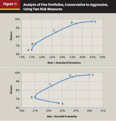
A different risk measure could alter what is considered the optimal asset allocation. As an example, for several years now, one of the risk metrics we use in asset allocation modeling is the probability that the portfolio will not beat inflation in the worst of the next several years. When calculating the efficient frontier using this version of a shortfall probability, and comparing it to an efficient frontier using standard deviation as the risk measure, the two graphs look reasonably similar. A portfolio that would be optimal using standard deviation would often be near-optimal using shortfall probability. The key exceptions are conservative portfolios. We find that the portfolios at the more conservative end of the efficient frontier using standard deviation are in the inefficient interior of the frontier when using shortfall probability as the risk measure. Figure 1 plots five selected portfolios, A through E—which span investment strategies conservative through aggressive, respectively—using the two alternative risk measures. This helps us quantify what we intuitively know—a portfolio that is “too conservative” runs a very high risk of losing value because of inflation. Calculating the shortfall probability and graphing the efficient frontier in this way helps us identify at what point a portfolio has become too conservative.

To more fully capture the dimensions of truly catastrophic risk, however, the investor wants to know not just the chance that the return will be below a certain threshold, but also how bad things may get when that happens. One way of calculating this fuller measure of risk is to use “conditional value at risk” (CVaR), which we recently added to our arsenal of risk metrics (we believe in using several risk metrics, not just one).
CVaR has long been used in the actuarial community to help determine insurance company capital requirements. It is an extension of the “value at risk” (VaR) concept, which is a common risk measure in the banking industry. VaR can be viewed as the answer to the question, “How bad can things get over a certain period?” You may calculate that for an investment as: there is a 5 percent chance of losing 25 percent of your principal of $10 million over a one-year period. The $2.5 million potential annual loss is the VaR of the investment at the 5 percent level. Another way to view VaR is as the inverse of shortfall probability. If the question is, “What is the probability of having a loss of $2.5 million or more?” the answer is 5 percent, and this is the shortfall probability. If the question is, “What is the value at risk at the 5 percent probability level?” the answer is $2.5 million, and this is the VaR.
CVaR can be a key metric in constructing portfolios that seek to avoid catastrophic losses. If VaR measures how bad things can get, CVaR answers the question, “How bad can it get when it gets bad?” CVaR is the conditional expected value of returns given that VaR has been breached. In the above example, we would focus on all the worst 5 percent possible scenarios. By focusing on this “left tail” of possible returns, we may find that one investment has never experienced a loss greater than 30 percent, and another investment has the potential to lose 65 percent of its value. Knowing the CVaR of these two portfolios would help you see that their risk profiles are actually quite different, which is something other risk measures may hide.
Although the CVaR of an individual investment is interesting, if you build well-diversified portfolios and rebalance regularly, it more appropriate to apply this metric on the portfolio level. In a well-diversified portfolio there may be individual assets with very high CVaRs. However, because of their countercyclical behavior relative to other assets in the portfolio, their inclusion actually causes the overall portfolio CVaR to decline. This last point is the crux of effective asset allocation. The goal of asset allocation from a risk management perspective is to identify the set of assets that offsets or mitigates each other’s risks, and to determine the optimal target allocation among them. Viewed in this context, it is not an asset’s individual risk-return profile that is of interest but rather its contribution to the profile of the overall portfolio. In order to properly evaluate this, it is crucial to understand the relationships among all assets within the portfolio over different market environments.
Estimating Relationships: Correlation Is Not Up to the Task
In our statistics classes we were taught that the relationship between two things can be measured by correlation, for which we were given the Pearson Rho formula. What most of us have not been taught is that not only are there numerous ways to calculate correlation, but correlation itself is often not a very good measure of the important relationships in many real-life applications.
One key flaw of any correlation formula is the implicit assumption that the relationship between two things is the same under all circumstances. This is generally not true, as it is clear that correlations change over time. It is particularly not true in turbulent regimes—asset classes that may have weak correlation during normal markets tend to have strong correlation during highly stressed markets. Another example is an investment that follows a buy-and-hold strategy (such as a long-only commodity index fund) versus one that uses a momentum strategy (such as managed futures). There may be very high positive correlation between these strategies during uptrending markets but negative correlation during declining markets.
What the preceding discussion points out is that the relationship between any two assets changes with how the assets themselves are performing. Instead of a single number to capture this relationship, it makes more sense to do so by means of a dynamic function. This allows the measure of the strength of the relationship to vary with the performance of the assets. A function such as this could easily capture low correlation during normal markets and high correlation during stressed markets. Once again, what may be new to most investment managers is old hat to actuaries. The relationship-as-dynamic-function concept is implemented via a copula dependency model,2 and has been used by actuaries for years.
A copula allows you to describe the dynamic relationship between two assets across the full range of their behavior. In particular, it allows that relationship to change based on the magnitude of each asset’s return. It thus provides an excellent solution to the problem of correlations becoming skewed during times of market stress.
Although the math behind a copula gets very complex very quickly, the idea behind it can be used quite easily for a heuristic understanding of relationships. To better visualize the relationship among assets, Figure 2 compares a long-only commodities index, the S&P GSCI Commodities Index, and a momentum-based commodities strategy, the Commodities Trends Indicator (CTI). CTI can go long or short individual commodity components depending on the momentum signals in its algorithm, and can be accessed via several publicly available investment vehicles. For the given example, we created a scatter plot on which each point represents the monthly returns of both indices for a given month. The S&P GSCI monthly return is measured along the x-axis, and the CTI monthly return is measured along the y-axis. For example, in the month labeled “A” on the graph, the return for S&P GSCI was –28 percent and the return for CTI was +19 percent.
Measured the traditional way, these monthly returns have a correlation of 24 percent over the entire period. This is consistent with the fairly high dispersion of the points around the diagonal line.3 However, note what happens at the two extremes. When commodities have very high returns, CTI’s returns are positive but relatively tame. When commodities do very poorly, CTI tends to outperform them to a significant degree. This would indicate that CTI is an excellent diversifier to long-only commodities—far more than is suggested by the 24 percent correlation. Viewing relationships between assets in this way allows you to visualize the relationship-as-dynamic-function concept captured by copulas.
Now imagine that, instead of a matrix of one-dimensional correlation coefficients to describe the interrelationships among all the assets in a portfolio, you replaced each of those numbers in the grid with a two-dimensional scatter plot such as the one in Figure 2. This should provide great insight into the strengths and weaknesses of your portfolios.
Copula dependency functions provide the math that allows you to incorporate these dynamic relationships directly into MPT.
Implementing the More Modern MPT
So far, we have discussed a few ideas on how to improve the inputs into the MPT portfolio optimization model. In this section, we focus on the model itself. Much of the software publicly available to calculate optimal portfolios makes many of the oversimplifying assumptions Markowitz made before the age of computers. The financial planning community should be demanding more.
One set of improvements is to allow for the more sophisticated inputs we have discussed—regarding risk, return, and relationships—to be incorporated in the model. As a model user, you should have the option to choose a probability distribution other than the normal to model returns; these distributions should accommodate asymmetry, skewness, and fat tails. You should have a suite of options for how you want to measure risk—a suite that includes shortfall probability and CVaR. And you should be able to use copulas to model relationships.
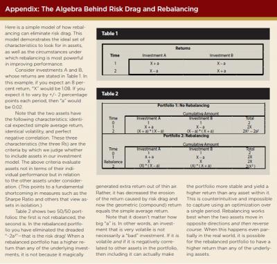
Perhaps the most fundamental change needed in software packages is in how they treat the investment horizon. Most portfolio optimizers assume that the user is investing over a single uninterrupted period. This is unrealistic and leads to two significant drawbacks: (1) the failure to recognize “risk drag,” and (2) the inability to reflect rules-based rebalancing.
Risk Is a Drag. Risk drag refers to the phenomenon that occurs when the volatility of an asset’s return over time erodes the compound return to the investor.
Compare the cumulative returns of two investments, each with an expected “average” return of 0 percent: one earns 0 percent each year and the other loses 10 percent one year and gains 10 percent the next. The cumulative return of the first investment is 0 percent. However, the cumulative return of the second investment is a loss of 1 percent. As this simple example demonstrates, any asset with volatility greater than zero will see its multi-year return eroded. And the more volatility, the more erosion. In fact, depending on its volatility, an asset with a high average return may not result in greater wealth than an asset with a lower average return but much less volatility. This difference between the simple average return and the compound return is the risk drag. And risk drag can be modeled only if your model assumes multiple time periods.
How important is risk drag as a practical matter? Consider the historical returns of the 10 S&P 500 industry sectors from 1990–2010. The financial sector had a simple average return of 11.3 percent, close to the 11.4 percent for the consumer staples sector, but a much lower compound return (7.7 percent versus 10.3 percent) because of its higher volatility. The most dramatic example of risk drag is information technology, which had a 15.5 percent simple average return, but, with the highest standard deviation of returns of any of the sectors, also had a risk drag of 5.5 percent, bringing its compound return down to 10.0 percent.
This presents a big problem. The appropriate measure of expected return in an MPT model is the simple average return over one period (typically a year), because that is what you are actually expecting to earn each year. When the MPT model views an investment horizon as a single period, it will simply adopt the expected mean return without regard to the effect of risk drag. It will therefore overstate the actual return over any realistic (longer) investment horizon. Making matters worse, the risk drag effect is not uniform across all asset classes, as our industry sector example shows, creating a severe problem when the primary purpose of the whole exercise is to determine optimal allocations among asset classes.
You might consider simply entering the compound annual return as the input instead of the simple average as a solution to this difficulty. There are numerous problems with this solution. One is that, all else equal, there is a different expected compound return for each multi-year investment horizon (the longer the horizon, the lower the return input should be—a particular problem if you are interested in seeing results over more than one horizon). Another is that the degree of risk drag is dependent on future volatility, which is something you’re projecting with the model and therefore not something you should be fixing deterministically in advance. See McCulloch (2003) for a comprehensive discussion of using simple versus compound returns in portfolio modeling. The most prominent problem for financial planners is that using geometric returns as the inputs in an MPT model doesn’t allow you to take the effects of rules-based rebalancing into account.
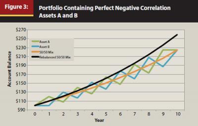
Rebalancing to the Rescue. Rebalancing can be thought of as the antidote to risk drag. (See the appendix for an algebraic explanation of risk drag and how rebalancing counters it.) Consider the following example, illustrated in Figure 3. Both asset A and asset B are very volatile, and they have perfect negative correlation with each other. When one zigs, the other zags—to exactly the same degree, but in the opposite direction. By diversifying between these investments, the investor can eliminate volatility without sacrificing return. But by diversifying and then rebalancing regularly, the investor can actually increase the portfolio’s return over time. The “extra” return is not generated out of thin air; it results from the decrease in the assets’ risk drag. In theory, rebalancing can eliminate risk drag; in practice it can at least reduce it.
So, here’s another problem. The most effective rebalancing algorithms are not those that rebalance at regular intervals, they are those that rebalance only when your asset allocations diverge from their targets by more than a tolerable amount. This is an example of what’s called rules-based rebalancing. With rules-based rebalancing, though you know the rules in advance, you cannot know the timing of your actual rebalancing until it happens. The future behavior of the individual asset classes will determine the timing.
Simulation-based, multi-period MPT models can easily handle this. Most portfolio optimization softwares today cannot, because they assume a single seamless period in their models. Why do we consider it necessary to be able to model real-time rules-based rebalancing? Because it reflects a critically important feature of how financial planners actually invest their clients’ portfolios. Without it, optimal portfolios are derived only by accident.
To be fair to the software vendors, this is a difficult feature to implement. There are formulas you can solve if you assume that there is only one period over which to optimize. When you no longer have that assumption, you no longer have neat solvable formulas either. The software would need to perform stochastic simulations. This is more complex than solving formulas and much more time-consuming, although there are algorithms to help speed this up (see Bernstein and Wilkinson (1998)). It’s also the most important improvement asset allocation programs can make.
The Time Is Now
The enhancements to MPT we cover here are overdue. There is simply no excuse for using 60-year-old technology when so much—your clients’ financial futures—is at stake. To not make these improvements is to be satisfied with exaggerated expected returns, sorely underestimated risk, and a deceptively high level of apparent diversification. The result is client portfolios that may look good on the screen but fail to hold up in the real world.
Although standard portfolio optimization software has not yet caught up with these improvements, there is no need for you to wait. We have implemented each of these improvements in our own shop, with homegrown, spreadsheet-based applications. When we needed help with certain technical aspects, we called in experts from the risk analytics community. Given that asset allocation is the single most important determinant of portfolio performance, the time and money we devoted to building our own model was well spent. This effort has been a high priority for us, and we are passionate about it. None of us, as financial planners, can afford to run the risk of finding ourselves unprepared for the next market calamity.
Endnotes
- See, for example, “What We Should Be Demanding from Our Asset Allocation Software,” a white paper written by Miccolis and Goodman and available at http://69.89.31.199/~brintone/wp-content/uploads/2010/09/BE-WhitePaper1.pdf; and The Kitces Report, December 2009 and January 2010, which Miccolis and Goodman co-wrote with Michael Kitces, available at www.kitces.com.
- In probability theory, the joint probability distribution of any two random variables can be decomposed into the marginal distributions of the two variables individually and a copula, which describes the dependence structure between the variables.
- If all the points fell along the diagonal line, the correlation would be +100 percent. The more dispersed the points are away from the diagonal, the more the correlation departs from 100 percent.
References
Bernstein, William J., and David J. Wilkinson. 1998. “Diversification, Rebalancing, and the Geometric Mean Frontier.” www.ssrn.com.
Chow, George, Eric Jacquier, Mark Kritzman, and Kenneth Lowry. 1999. “Optimal Portfolios in Good Times and Bad.” Financial Analysts Journal (May/June).
Markowitz, Harry. 1952. “Portfolio Selection.” Journal of Finance (March).
McCulloch, Brian W. 2003. “Geometric Return and Portfolio Analysis.” New Zealand Treasury Working Paper No. 03/28 (December).