Right-Sizing Retirement

Journal of Financial Planning: February 2021

 

Executive Summary

• Research suggests some households underspend in retirement, resulting in a “retirement consumption gap.” This paper explores this effect, specifically during the first 10 years of retirement, and incorporates both household assets and pre-retirement spending using data from the Health and Retirement Study.
• Only 18 percent of households have enough wealth to cover pre-retirement consumption when they retire, which suggests most households will not be able to maintain their pre-retirement lifestyle in retirement—a finding consistent with other general estimates of the retirement readiness of Americans.
• Real financial assets decline for 65 percent of households during the first 10 years of retirement, with a median real decline of 35 percent.
• Real retiree spending declines for 75 percent of households during the first 10 years of retirement, with a median annual decline of approximately 2 percent per year. This suggests financial planners should consider changes in retirement spending that are less than inflation as part of a retirement plan.
• The percentage of households that can fund their retirement consumption increases dramatically during the first 10 years of retirement, from 18 percent to 48 percent, primarily due to reductions in spending. This suggests households “right-size” their spending early in retirement to better align with available resources. It is not clear, though, to what extent this behavior persists further into retirement (due to data limitations).
• Many well-funded households could increase consumption, but appear not to do so (i.e., exhibit a retirement consumption gap). Potential reasons include the desire to leave a bequest, uncertain medical expenses (especially late in retirement), uncertain life expectancy, etc. While this group is a minority of retiree households, understanding what drives this behavior is especially important to financial planners since this group tends to have the most accumulated wealth and are, therefore, more likely to seek the services of, or use, a financial planner.

David M. Blanchett, Ph.D., CFA, CFP^®, is head of retirement research at Morningstar Investment Management and an adjunct professor of wealth management at The American College of Financial Services. He is the recipient of the Journal’s 2007 Financial Frontiers Award and its 2014, 2015, and 2019 Montgomery-Warschauer Award.

Warren Cormier is executive director of the Defined Contribution Institutional Investment Association (DCIIA) Retirement Research Center (RRC). He has previously served as CEO and co-founder of Boston Research Technologies. He is also the co-founder of the RAND Behavioral Finance Forum dedicated to helping consumers make better financial decisions.

NOTE: Click or tap on images below for PDF versions of the Figures and Tables. 

JOIN THE DISCUSSION: Discuss this article with fellow FPA Members through FPA's Knowledge Circles​​​​. ​​​

FEEDBACK: If you have any questions or comments on this article, please contact the editor HERE. 

Research suggests there is a number of retiree households that underspends, resulting in a “retirement consumption gap” (Browning et al. 2014). The idea that retiree households under-consume has important policy implications, as well as implications for retirement savings in general: why save for retirement if you’re not going to spend it? Most research exploring this effect has focused primarily on retirement asset levels—for example, whether assets are being depleted and the extent the depletion would be considered optimal, or used surveys of retiree households but has not also considered pre-retirement spending (i.e., the retirement liability) when noting the effect.

This research explores the retirement consumption gap and considers both the wealth available to fund retirement, defined as either financial assets, such as a taxable account or an IRA, or guaranteed income such as Social Security retirement benefits, a private pension or annuity, and spending, or consumption, both before and after retirement. Considering both the assets and the pre-retirement spending provides a much richer context around spending decisions during retirement. The analysis used data from the RAND Health and Retirement Study and focused specifically on changes in spending during the first 10 years of retirement.¹ 

There are numerous key findings. First, only 18 percent of households were estimated to have enough wealth to cover pre-retirement spending during retirement. Second, most retirees spend down financial assets, but at different rates. Median real financial assets were 35 percent lower 10 years following retirement and 65 percent of households had fewer assets 10 years after retiring, in today’s dollars.² Households with the lowest initial funded ratios³ tended to spend down financial assets the most, relatively speaking, and had the fewest assets, initially (in absolute terms).

Third, spending declined in real terms over the first 10 years of retirement for 75 percent households, with a median total reduction of 23 percent (i.e., approximately 2 percent per year). This effect has been noted in past research (Blanchett 2014, among others) and has important implications when forecasting retirement spending in a financial plan since most planners assume retiree spending increases annually with inflation throughout retirement (although it does, empirically, on average). Finally, the percentage of households that can fund their retirement consumption (i.e., have a funded ratio of one or greater) increases dramatically during the first 10 years for retirement, from 18 percent to 48 percent. This shift is largely a result of reductions in spending, especially among households with the lowest initial funded ratios, and suggests that households, at least in early retirement, attempt to “right-size” their spending to better align with available resources.

Perhaps the most interesting households in the analysis are those that have more than enough wealth to cover pre-retirement spending (i.e., a funded ratio greater than 1.0). This group is especially relevant to financial planners because they tend to have accumulated the most financial wealth and, therefore, are more likely to need help managing these assets—and are more desirable as clients since there are more assets to manage. While these well-funded households are the minority,⁴ 29 percent have more wealth, in today’s dollars, 10 years after retirement, and 54 percent have funded ratios that increase (at least slightly) over the period of study. These well-funded households could increase consumption but appear to choose not to do so. As previously discussed, uncertainty, regret, and difficulty with temporal effects explain some of the underspending. There are likely other factors driving underspending that cannot easily be observed in survey data, such as the desire to leave a bequest. Understanding the financial behaviors of this group will be an important strand of literature going forward.

Overall, this analysis suggests that any type of retirement consumption gap observed early in retirement can likely be explained by households attempting to match resources to available spending (i.e., “right-sizing” their consumption). Importantly, 69 percent of all households improve their funded ratio in retirement; 75 percent of households with initial funded ratios less than 1.0 improve their funded ratio in retirement.

It is not clear, though, to what extent this gap persists further into retirement—for example by year 15 or 20. It could be that households that are forced to “right-size” during the first 10 years of retirement continue to reduce spending, even though they may not need to (i.e., the belt continues to tighten) and evidence of reduced spending by well-funded households suggests this may be the case. Regardless, the relatively poor funded status of most households suggests that pre-retirees should focus on saving more for retirement, although traditional approaches to estimating required retirement savings may be overstating the actual amount needed based on various observed behaviors (i.e., spending declines in real terms and over-funded households tend to under-consume).

Literature Review

Retirement is the largest expenditure that most households ever make, yet its cost is effectively unknown until it is fully experienced (i.e., death). The fundamental uncertainty regarding the cost of retirement makes it especially difficult to save for, especially at the individual household level, given the idiosyncratic risks that exist at the individual household level.

The life-cycle hypothesis, which was introduced initially by Modigliani and Brumberg (1954), implies that individuals plan their savings and consumption behavior in order to smooth out their consumption over their entire lifetime, thereby, maximizing their expected lifetime utility. A key assumption is that individuals prefer stable lifestyles versus volatile lifestyles. The optimal consumption path is going to vary by individual/household, and is determined based on things like the utility parameters, discount rate, mortality risk, expected future compensation, etc.

Errors in key assumptions around retirement spending could lead to over- or under-saving. For example, spending is commonly assumed to increase with inflation during retirement, despite empirical evidence that retiree spending tends to decline (in real terms). Stein (1999) noted that retirees exhibit “go-go, slow-go, and no-go” phases of retirement, where younger retirees enjoy a more active retirement where spending declines as retirees age based on health, an effect that has been documented empirically by Blanchett (2014), among others. If a household bases saving decisions on the assumption that spending will increase annually by inflation during retirement, but it eventually does not, it may over-save, on average.

Browning, Guo, Cheng, and Finke (2016) noted that households with a de minimis level of assets (approximately $10,000) have a consumption gap of approximately 8 percent, on average, while households with higher levels of wealth exhibit a consumption gap as high as 53 percent. Even after considering spending risks and bequests, a significant spending gap is noted to persist.

De Nardi, French, and Jones (2016) noted that retired U.S. households, especially those with high income, decumulate their net worth at a slower rate than that implied by a basic life-cycle model in which the time of death is known. Poterba, Venti, and Wise (2011) explored the “potential additional annuity income” that households could purchase, given their holdings of non-annuitized financial assets at the start of retirement, and found that 47 percent of households between the ages of 65 and 69 in 2008 could increase their life-contingent income by more than $5,000 per year. They noted the effect is especially pronounced at the upper end of the wealth distribution.

Banerjee (2018) noted that while most retirees do spend down their assets in the first 18 years following retirement, about one-third of all sampled retirees had increased their assets over that period. It is not necessarily clear why some households seem averse to accessing savings to fund consumption. The Society of Actuaries⁵ interviewed retirees and concluded that respondents wanted to maintain or increase asset levels, and this was primarily accomplished through cuts in spending (an effect observed in this research).

While housing is an asset that could be used to fund retirement, and research suggests it can improve retirement outcomes (Pfau 2016), retirees appear to have relatively little interest in accessing home equity according to Poterba, Venti, and Wise (2011), Fisher et al. 2007, and others. A survey conducted by the Society of Actuaries⁶ noted that only 11 percent of retired respondents indicated that they were planning to use home equity to finance their retirement.

There are several potential reasons to explain why some retirees under-consume, such as the desire to leave a bequest, uncertain medical expenses (especially late in retirement), and uncertain life expectancy. However, research attempting to control for these effects suggests a retirement consumption gap still exists for some households. For example, only 25 percent of retirees are noted to have an explicit bequest motive (Browning 2018) and while medical expenses at advanced ages can be incredibly expensive, such as an extended stay in a nursing home facility, for most retirees they are not (Nordman et al. 2016). Focusing on the tail risk associated with medical costs and self-insuring is clearly suboptimal and suggests a private option, such as purchasing long-term care insurance, or some type of new government (public) program, could benefit retirees.

The idea of a retirement consumption gap seems slightly at odds with the general picture of retirement readiness in America. There is a large body of research, going back decades, noting that most U.S. households are poorly positioned to fund retirement (Bernheim 1993; Munnell and Soto 2005; Mitchell and Moore 1998). For example, the Center for Retirement Research at Boston College noted that approximately 50 percent of households are “at risk” of not having enough to maintain their living standards in retirement, based on National Retirement Risk Index⁷ and EBRI noted 40.6 percent of U.S. households are projected to run short of money in retirement based on its Retirement Security Projection Model.⁸ How can retirees have under-saved and then not spend what little monies exist?

This research seeks to at least provide some context around this question and suggests these two facts are actually related, at least in early retirement: households actively decide to spend less in early retirement to “right-size” spending with available resources, or to prolong what little resources that are available. The extent that early reductions in consumption persist later in retirement could explain the broader effect noted at older ages, especially since many retirees who have accumulated enough wealth appear to under-spend.

Dataset

The analysis is conducted using data from the Health and Retirement Study (HRS). The HRS is a longitudinal household survey conducted by the Institute for Social Research at the University of Michigan that surveys a representative sample of approximately 20,000 people in America, and supported by the National Institute on Aging and the Social Security Administration. It has been administered on a biennial basis since 1992. This analysis uses income, assets, and demographic data specifically from the RAND HRS Longitudinal File and spending (i.e., consumption) from the RAND CAMS Spending Data. The RAND HRS Longitudinal File is a user-friendly version of a subset of the HRS and the RAND CAMS is a user-friendly version of Part B of the CAMS survey.

The definition of spending for the analysis is household consumption, which is estimated by RAND. Consumption is used as the metric for spending, versus other potential measures (e.g., total spending) since it attempts to smooth the useful life of various durable goods over their respective usage periods. The analysis uses waves five through 13 of the respective surveys, covering years 2001 to 2015.

The assumed retirement year is the closest survey year to the respondent’s retirement age, if the household is a couple (i.e., based on the age of the second member to retire). Therefore, while the first wave used for each household is called “retirement,” it may be slightly before or after the household retires, given differences in survey data (i.e., it’s biennial), especially for households with members who retire in different years.

A number of filters are applied to the households included the analysis. First, a household must be coded as becoming retired during the waves reviewed. If the household is a couple, both members must be coded as retiring during the available waves and both must retire within three years. Pre-retirement year consumption must be greater than or equal to $10,000, based on the assumed year of retirement. The pre-retirement consumption can average up to three waves of consumption data, adjusted for inflation, if available, in order to smooth out potential changes. The retiree household must have at least $10,000 in pre-retirement assets. The household must claim Social Security benefits during the period available, and total benefits must be greater than $5,000. Additionally, consumption data must be available for at least the wave following assumed retirement. All values are converted into real terms based on the assumed year of retirement for each household.

A total of 425 households met the required filters to be included in this analysis. Pre-retirement consumption (R₀) is compared to up to five subsequent waves, which would be plus two years (R + 2), plus four years (R + 4), plus six years (R + 6), plus eight years (R + 8), and plus 10 years (R + 10) following retirement. Required data for all fields varies by post-retirement period and there were 425 households that met the necessary requirements for R + 2 (this is a requirement to be included in the dataset), 357 households for (R + 4), 302 households for (R + 6), 233 households for (R + 8), and 167 households for (R + 10). One reason the number of households declines over longer post-retirement periods (e.g., R + 10) is due to later waves being used and, therefore, data not being available yet. A household could be missing data for a future period but be included in other years [e.g., if consumption was missing for (R + 4), the household could still be included in (R + 6), (R + 8), and (R + 10), if available]. The distribution of households by assumed CAMS year of retirement years 2001, 2003, 2005, 2007, 2009, 2011, and 2013 are 71, 90, 64, 67, 54, 43, and 36, respectively (there must be consumption for at least one year of retirement, which is why retirement is never assumed to occur in 2015).

A key metric used to estimate the likelihood of a household being able to fund future consumption is the funded ratio. The funded ratio metric is calculated by adding the existing level of guaranteed income to an estimate of the amount of income the portfolio could generate based on the expected duration of retirement for the household and dividing this total by the current level of consumption.

The funded ratio used for the analysis is really is more of an income replacement metric since it the expected level of Social Security benefits, plus pension and annuity income for that year, plus an estimate of income that can be generated from:

 

 

The effective tax rate is estimated based on the composition of assets to determine the approximate taxes required to generate the target consumption level (which is after taxes). This research uses 2019 tax brackets, standard deviations, and tax rates for simplicity purposes, but adjusts the respective breakpoints to the actual year of analysis. Note: Social Security retirement benefit taxation levels have not changed since the Omnibus Budget Reconciliation Act passed in 1993. Total effective tax rates vary primarily based on the total level of consumption and the extent of Social Security retirement benefits. Overall effective rates are relatively low, averaging only about 7 percent over the period of analysis.

 

 

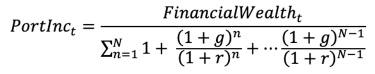
The portfolio income amount is effectively divided by the present value factor of an annuity due where the payments are assumed to increase by some constant growth rate (g), which is assumed to be 2 percent. The time period (N) is set so that the household only has a 25 percent probability of outliving it, where mortality is based on the Social Security Administration’s 2007 Period Life Table.⁹ The mortality calculations are based on household composition (i.e., incorporates whether it is a single or joint household and the respective ages and genders). The 2007 Period Life Table is used since it represents the approximate mid-point of retirement for the analysis (from 2001 to 2015). The discount rate is the yield on the long-term government bonds for the respective year (r), defined as the Ibbotson Associates SBBI U.S. Long-Term Government Bond Index. The pricing model is similar to how an immediate annuity with a fixed cost of living adjustment would be priced, except a slightly longer period is used because the household is assumed to self-annuitize and, therefore, would want an implied probability of less than 50 percent of outliving the respective planning period.

Other funded ratio metrics commonly include mortality weighted net present values for things like guaranteed income and spending. A simpler approach is used here since it requires fewer assumptions about future growth rates and future spending and likely better corresponds to how households think about overall fundedness. One shortfall of the approach used is that it does not consider the different cost of living adjustments associated with different types of income (e.g., Social Security retirement benefits are linked to inflation while pension benefits are commonly not).

Home equity is excluded as a financial asset in the funded ratio because it is not commonly used by households to fund retirement (as noted in the Literature Review section). Therefore, the funded ratio is focused entirely on the financial wealth available to fund retirement, which includes investment accounts, such as a taxable accounts and IRAs, as well guaranteed income sources, such as Social Security retirement benefits, pension benefits, etc.

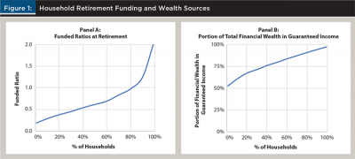
Households are placed into four groups based on their funded ratio at retirement: <0.5, 0.5 to 0.75, 0.75 to 1.0, and greater than 1.0. A household with a funded ratio greater than 1 would be assumed to have more than enough wealth to fund consumption. Figure 1 includes information about the distribution of funded ratios at retirement (Panel A) and the distribution of guaranteed income as a percentage of total wealth for the available households (Panel B).

 

 

There is a general positive correlation between funded status and self-reported retirement satisfaction among households. The relation is only statistically significant for the (R + 8) period, though, with a p-value of .0044 (based on a univariate regression where the dependent variable is self-reported retirement satisfaction, and the independent variable is the funded ratio). The statistical significance of the relation decreases significantly, though, when other household attributes are controlled for, such as age (older households tend to report higher levels of satisfaction) and, especially, health (health is positively correlated to retirement satisfaction).

There is quite a bit of literature documenting the positive relation between health and wealth (Smith 1999 and Poterba, Venti, and Wise, 2010); therefore, it is important to consider health when considering the role of funded status (since there is a correlation between wealth and health). The coefficient for funded ratio is still statistically significant when these other variables are controlled for, but just barely (p-value of 0.0497). Therefore, while there does appear to be a positive relationship between funded ratio and retirement satisfaction—for example better-funded households are happier—the statistical significance is weak and warrants further exploration

Consistent with other literature on the topic of retirement readiness, most households are estimated to not have adequate wealth to fund pre-retirement consumption at retirement, with only 18 percent of households estimated to have a funded ratio greater than or equal to one. Guaranteed income sources are the predominant asset households have to fund retirement, representing between 50 percent and 100 percent of the household’s total financial wealth.

A series of ordinary least squares (OLS) regressions are performed as part of the analysis. For each regression the dependent variable is the change in the respective value under consideration, which is real total assets (Table 1), real total spending (Table 2), or the funded ratio (Table 3) for a future retirement period (R + 2 to R + 10). The dependent variable is bounded between –100 (a 100 percent drop) and 100 (a 100 percent increase) to minimize the impact of outliers.

 

 

 

 

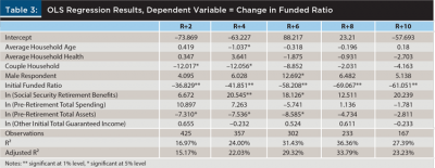
Independent variables included in the regressions are: average household age at retirement, average household health at retirement, whether the household is a couple at retirement (this is a dummy variable, set to 1 if the household is a couple, otherwise it’s 0), whether the respondent is a male, the initial funded ratio, the natural logarithm of Social Security retirement benefits, the natural logarithm of pre-retirement spending, the natural logarithm of pre-retirement total assets, and the natural logarithm of other initial guaranteed income. All regressions included household weights, based on the R₀ year values. The households included in the regressions vary by respective future retirement year (e.g., (R + 2) versus (R + 6) but are the same for each of the three sets of regressions. The regression results and discussions are considered, along with other information around the respective text.

Analysis

To understand whether households exhibit a retirement consumption gap in early retirement, the first thing to explore is how financial assets evolve over the period. If financial assets increase during early retirement, that would be strong evidence that households do not use accumulated wealth to fund retirement and would provide evidence of a retirement consumption gap. However, households do appear to be depleting financial assets since they decline in both absolute terms (Panel A) and relative terms (Panel B) during the first 10 years of retirement, for each of the four funded ratio groups considered in the analysis, as demonstrated in Figure 2.

 

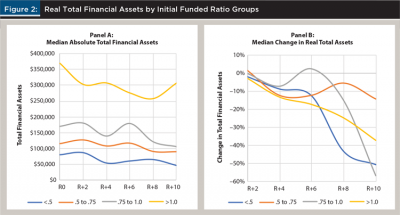
While only 51 percent have lower financial assets for the first post-retirement wave [i.e., (R + 2), which is two years following retirement], 65 percent of households have fewer assets 10 years into retirement, in real terms. Households with the lowest funded ratios tend to have the fewest initial assets upon retirement (which is the key driver of the low-funded ratio) as well as a relatively faster depletion over time.

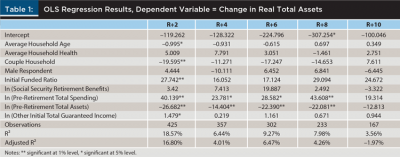
The OLS regression results where the dependent variable is the change in total real assets are included in Table 1.

The results imply that real financial assets fell more for households with higher levels of initial spending and then less for those lower initial asset values (controlling for all other factors). The spending relation is expected since higher levels of spending represent an outflow that will reduce assets. The negative coefficient for assets is somewhat contrary to the information in Panel B and suggests those with the least amount of savings were less willing to spend from existing savings.

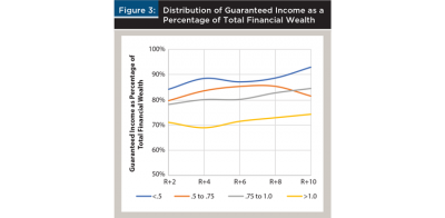
Since financial assets decline during the first 10 years of retirement, at least on average, the relative role of guaranteed income, as a percentage of total wealth, is likely to increase. This effect is demonstrated in Figure 3, which includes the distribution of guaranteed income as a percentage of total financial wealth during the first 10 years of retirement. The estimates used for this calculation are the same for the funded ratio, where an estimate of the potential income that can be generated from the portfolio is compared to the respective annual income generated from guaranteed income sources.

Figure 3 suggests guaranteed income is a significant asset for retirees, especially among those who have lower funded ratios (i.e., fewer financial assets). Even for the highest funded ratio group, roughly 70 percent of total financial wealth is in some form of guaranteed income for the median household. Within each funded ratio group there are going to be significant differences, though.

 

 

Next, real consumption is explored for the funded ratio groups for the first 10 years of retirement, and the results are included in Figure 4 in both absolute (Panel A) and relative terms (Panel B).

 

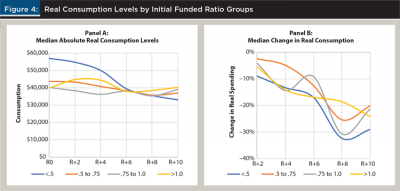
Households with the lowest funded ratios tend to have the highest levels of initial consumption, but consumption levels of all groups tend to roughly converge by year 10. The percentage of households spending less declines monotonically by year, with 41 percent spending less by (R + 2), 35 percent by (R + 4), 32 percent by (R + 6), 26 percent by (R + 8), and 25 percent by (R + 10) (i.e., 75 percent of households are spending less, in today’s dollars, by year 10 of retirement).

While the households with the lowest initial funded ratios had the largest drop in consumption, all groups exhibited reductions in real spending. The median total change in real spending over the first 10 years of retirement is –23 percent, which suggests spending is declining by roughly the inflation over the period (i.e., 2 percent a year, where spending is constant in nominal terms). While this is consistent to some extent with past research on the topic (Blanchett 2014), it does not align with generally expected behavior. In theory, households with sufficient assets to fund consumption can continue spending at the same level, and we would expect relative changes in the groups to be relatively monotonic by funded ratio (i.e., those who have the highest funded ratios reduce spending by the least, or possibly increase spending).

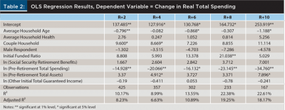
The results of the OLS regressions are included in Table 2 and suggest that spending tended to decline the most for older retirees who were single, with higher spending levels, holding everything else constant.

The noted reduction in real spending is somewhat at odds with common financial planning assumptions, where retirement spending is generally assumed to increase annually with inflation. The fact that spending declines for households—even for those who are not resource constrained (i.e., have funded ratios exceeding one)—suggests that assuming retirement spending increases annually is something that should be reconsidered by financial planners.

While retiree households appear to be depleting assets, which reduces the funded ratio, they also appear to be reducing spending, which increases the funded ratio. Therefore, the overall implications on how funded ratios evolve is ambiguous. If financial asset declines exceed the relative drop in spending, funded ratios could decrease into retirement, and the reverse could also be true.

Figure 5 illustrates how funded ratios evolve during the first 10 years of retirement by initial funded ratio group (Panel A) as well as the percentage of households with a funded ratio greater than or equal to one (Panel B).

 

 

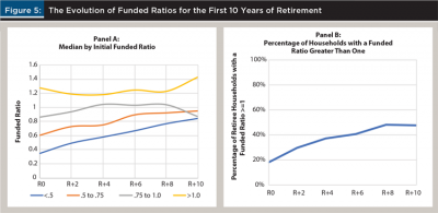
The median funded ratio of all households increases from .61 to .94, and funded ratios effectively increase for all initial funded ratio groups during the first 10 years of retirement. Households with the lowest initial funded ratios (less than .5) see the greatest improvement in their funded ratios, increasing from a median of .35 to .84. Eighty-eight percent of households in the lowest funded group (<.5) have increased their funded ratios after 10 years, compared to 76 percent in the next group (.5 to .75), while the two groups that are closer to fully funded are effectively unchanged. Perhaps most notably, the percentage of households that appear to be fully funded (i.e., a funded ratio greater than or equal to one) increases from 18 percent to 48 percent over the 10-year period.

The results of the OLS regressions are included in Table 3 and suggest that funded ratios tend to rise the most for those households with the lowest initial funded ratios with the least initial assets. This is consistent with the results in Figure 5, which suggest those households that are in the worst shape initially see the most improvement during the first 10 years of retirement.

The notable improvement in funded ratios suggests that households try to “right-size” their retirement spending to a more reasonable level given available assets in early retirement. Therefore, the fact that retirees may not appear to be consuming optimally is more a function of ensuring the assets better reflect spending (i.e., the liability) versus simply deciding to not consume. It is not clear, though, to what extent this effect continues beyond the tenth year of retirement. If households continue to reduce spending (which is likely given other research on retiree spending behaviors), funded ratios could continue increasing, creating a retirement consumption gap for the majority of households (versus just those who are well-funded).

What’s Driving the Improvement in Funded Ratios for Retiree Households?

There are effectively five key variables to the funded ratio calculation: total financial assets, estimated payout rate for financial assets, guaranteed income, effective tax rate, and consumption. The guaranteed income portion is relatively fixed over time since Social Security retirement benefits are assumed for all periods. The effective tax rate is going to vary primarily based on the level of consumption because guaranteed income is assumed to be fixed. The estimated payout rate for financial assets is exogenous by the level of assets and depends on household structure and respective retirement year. Therefore, changes in the funded ratios are going to be primarily driven by changes in spending and asset levels.

To try to determine whether changes in financial assets (i.e., spending down assets) or spending (i.e., the liability) are resulting in changes to the funded ratio, an additional analysis is performed. For the analysis, either the initial consumption or total financial assets is held constant, while the other attributes are assumed to vary. This creates two alternative funded ratio paths for the retiree household. The respective paths are weighted (between 0 percent and 100 percent, in 10 percent increments) and compared to the actual funded ratio path for the household (i.e., how the funded ratio actually evolves in retirement). The weights that result in the smallest deviation or, more technically, the smallest sum of the squared errors, is deemed to provide some perspective on whether assets or savings are the primary driver of changing funded ratios.

The resulting metric is the percentage of change in the funded ratio that can be attributed to changes in spending levels. The remainder (i.e., one minus the value) would be the amount attributed to changes in financial assets. This is obviously an imperfect approach but provides some way to quantify the relative contribution of changes to the two key drivers the household controls, with respect to its funded status. The distribution of the results for each funded ratio group is included in Table 4.

 

 

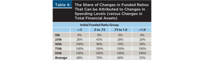
Changes in spending levels are estimated to be the primary driver of changes in funded ratios, driving approximately 65 percent of the estimated change in funded ratios. The relative importance of spending changes is more important for households with lower funded ratios. This is not all that surprising given the relatively low financial assets noted for these households in Figure 1.

Conclusions

Retirement is the most expensive purchase most individuals ever make; therefore, it is especially important to understand its cost and save appropriately. This research suggests that while many retirees do reduce consumption early in retirement, the effect may be related more to necessity than choice. This also suggests that there may be possible refinements to retirement planning processes that would help people understand the realities of spending in retirement as opposed to being surprised after they have actually retired. Future research will hopefully explore this effect in greater detail to help better understand the motivations and decisions of retirees and paint a more complete picture of retirement.

Endnotes

1. Technically, the first five HRS waves follow retirement. The period of analysis (10 years) is limited because the CAMS survey has only been sent out since 2001 and consumption data is only available through 2015.
2. Among those with at least $10,000 in total financial assets at retirement, this was an initial filter for the analysis.
3. This can generally be defined as the total assets available to fund retirement, divided by retirement income need. The higher the number, the better able the retiree household is to fund its spending.
4. Only 18 percent of those considered, and the actual proportion within the U.S. population is likely smaller given the constraints imposed on the households included in the analysis.
5. See The Society of Actuaries 2009 Risks and Process of Retirement Survey: Report of Findings.
6. Ibid.
7. See crr.bc.edu/special-projects/national-retirement-risk-index/.
8. See www.ebri.org/content/retirement-savings-shortfalls-evidence-from-ebri-s-2019-retirement-security-projection-model.
9. See www.ssa.gov/oact/STATS/table4c6_2007.html.

References

Banerjee, Sudipto. 2018. “Asset Decumulation or Asset Preservation? What Guides Retirement Spending?” EBRI Issue Brief, No. 447. Employee Benefit Research Institute.

Bernheim, B. Douglas. 1993. “Is the Baby Boom Generation Preparing Adequately for Retirement?” Merrill Lynch.

Blanchett, David M. 2014. “Exploring the Retirement Consumption Puzzle.” Journal of Financial Planning 27 (5): 34–42.

Browning, Christopher, Tao Guo, Yuanshan Cheng, and Michael S. Finke. 2016. “Spending in Retirement: Determining the Consumption Gap.” Journal of Financial Planning 29 (2): 42–53.

Browning, Christopher. 2018. “Post-Retirement Spending Discomfort and the Role of Preparedness, Preferences, and Expectations.” Journal of Personal Finance 17 (2): 51–61.

De Nardi, Mariacristina, Eric French, and John B. Jones. 2010. “Why Do the Elderly Save? The Role of Medical Expenses.” Journal of Political Economy 118 (1): 39–75.

Fisher, Jonathan, David Johnson, Joseph Marchand, Timothy Smeeding, and Barbara Boyle Torrey. 2007. “No Place Like Home: Older Adults and Their Housing.” The Journals of Gerontology Series B: Psychological Sciences and Social Sciences 62 (2): S120–S128.

Mitchell, Olivia S., and James F. Moore. 1998. “Can Americans Afford to Retire? New Evidence on Retirement Saving Adequacy.” Journal of Risk and Insurance 65 (3): 371–400.

Modigliani, Franco, and Richard Brumberg. 1954. “Utility Analysis and the Consumption Function: An Interpretation of Cross-Section Data.” In Post-Kenyesian Economics, edited by Kenneth K. Kurihara. New Brunswick, N.J.: Rutgers University Press.

Munnell, Alicia, and Mauricio Soto. 2005. “What Replacement Rates Do Households Actually Experience in Retirement?” Available at SSRN 1150172.

Nordman, Eric C., John Ameriks, Vincent Bodnar, Joseph Briggs, Bonnie Burns, Laura Cali, Andrew Caplin et al. 2016. “The State of Long-Term Care Insurance: The Market, Challenges and Future Innovations.” National Association of Insurance Commissioners and The Center for Insurance Policy and Research.

Pfau, Wade D. 2016. “Incorporating Home Equity into a Retirement Income Strategy.” Journal of Financial Planning 29 (4): 41–49.

Poterba, James M., Steven F. Venti, and David A. Wise. 2010. “The Asset Cost of Poor Health.” No. w16389. National Bureau of Economic Research.

Poterba, James, Steven Venti, and David Wise. 2011. “The Composition and Drawdown of Wealth in Retirement.” Journal of Economic Perspectives 25 (4): 95–118.

Smith, James P. 1999. “Healthy Bodies and Thick Wallets: The Dual Relation Between Health and Economic Status.” Journal of Economic Perspectives 13 (2): 145–166.

Stein, Michael K. 1998. The Prosperous Retirement: Guide to the New Reality. Emstco Press.

Citation

Blanchett, David M., and Warren Comier. 2021. “Right-Sizing Retirement: Exploring the Retirement Consumption Gap in Early Retirement.” Journal of Financial Planning 34 (2): 68–81.