Journal of Financial Planning: February 2019
Executive Summary
- Financial advisers with an investment emphasis may commonly suggest that pre-retirement life insurance needs are best met by using a “buy term and invest the difference” strategy that pays the smallest premiums for a temporary death benefit, allowing more assets to be invested.
- Investments, however, may not be ideally suited for managing the full range of post-retirement financial risks, including longevity risk, market volatility, and spending shocks.
- This study considers whole life insurance as an alternative to “buy term and invest the difference” as part of a lifetime financial plan.
- Three possible uses of whole life insurance in a lifetime financial plan for a hypothetical couple, both age 40, are investigated.
- The analyses suggest that integrating whole life insurance into a lifetime financial plan has the potential to allow a given asset base to support greater lifetime spending and greater legacy than “buy term and invest the difference” strategies.
Wade D. Pfau, Ph.D., CFA, is a professor of retirement income at The American College and a principal at McLean Asset Management. He also works as chief planning strategist for inStream Solutions. He is a two-time recipient of the Journal’s Montgomery-Warschauer Award. He hosts the Retirement Researcher website (www.RetirementResearcher.com).
Disclosure: The strategy described in Table 2 is based on an earlier research project by the author that was funded through OneAmerica (which offers a range of whole life insurance products) and published as “Optimizing Retirement Income by Combining Actuarial Science and Investments” in 2015 in the Retirement Management Journal, 5 (2): 15–32.
The traditional purpose of life insurance is to provide a death benefit to help support surviving family members or a family business in the event of the policyholder’s untimely death. The amount of life insurance one seeks to hold is typically the amount dependents would need to sustain their lifestyle or meet their obligations in the absence of the policyholder contributing to the family through wages or other caretaking. For this basic human capital replacement framework, one generally does not associate a need for life insurance after retirement begins.
Term life insurance can successfully serve the role of human capital replacement. Because the death benefit is temporary with term life insurance, and it does not include a savings component, the premiums for term life are smaller than other forms of life insurance. For a given pool of funds, this affords a greater remaining amount to be invested after life insurance obligations are met. A mantra of “buy term and invest the difference” has developed as the way to approach the life insurance decision.
But for lifetime financial planning, is it best to pay the smallest amount possible for life insurance in order to invest as much as possible in the financial markets? This research put the concept of “buy term and invest the difference” to the test by comparing it with strategies that include permanent whole life insurance as part of a longer-term retirement strategy that can be set into motion during the accumulation phase. Which approach can obtain the most spending power and legacy from an available asset base?
This study investigated three ways a couple could consider incorporating whole life insurance into their lifetime financial plan: (1) as an alternative means for funding a legacy goal; (2) as a behavioral justification for also including an income annuity in their retirement plan; and (3) as a volatility buffer to help manage sequence of returns risk for their investments.
Literature Review
The conventional wisdom in the investment world is that an individual’s life insurance needs are best served by paying a smaller premium for term insurance, which allows more to be invested for growth over time. With a sufficiently high rate of return assumption for investments, this approach can support greater net wealth accumulations. No published research, known to the author, has demonstrated this point; rather, it is commonly expressed as an article of faith that investments will outperform cash value accumulation, net of fees.
Published research about cash value life insurance has generally suggested that the beneficial aspects for permanent life insurance may be overlooked in the conventional wisdom. Smith (1982) described a whole life insurance policy as a complicated set of financial options that cannot be replicated with other investments. Babbel and Hahl (2015) found insufficient basis for the conclusion that “buy term and invest the difference” is a dominant strategy. A 2017 Morningstar white paper1 examined the 35-year performance of a whole life insurance policy and found that the internal rate of return on its cash value was comparable with other bond investments, and that this outcome was provided with less volatility. Fechtel (2012) provided an educational approach to clarify how permanent life insurance works in order to better compare it with buy term and invest the difference alternatives.
Within the world of retirement income planning, whole life insurance has been investigated in a few ways. Pfau (2015) described a strategy in which whole life insurance is combined with a single-life immediate annuity and investments to support greater retirement efficiency in terms of spending and legacy.
Teitelbaum (2014) provided a common example of using the cash value of life insurance as a volatility buffer in retirement. One draws from the cash value to sustain spending in years after market downturns with the same decision rules used by Sacks and Sacks (2012) to describe the Home Equity Conversion Mortgage (HECM) as another type of volatility buffer. However, Teitelbaum introduced an additional asset to the investment portfolio such that the positive impact of the cash value insurance can be ascribed having more assets available to reduce the overall distribution rate. To be an effective volatility buffer, it is important that reductions to other investment assets, as well as the unique performance of the cash value, must be accounted for as part of the process to create the cash value buffer asset.
Pricing Policies: Economic Framework, Simplifications, and Assumptions
This study used a simplified economic framework to compare investment and insurance strategies on an equal basis. Simplifications included certainty about future population mortality rates, interest rates, and company expenses. This was done so that life insurance premiums did not need to build in reserves that were returned as dividends when worst-case assumptions were not met. (Assumptions for investment returns are explained in the case study section.)
Life insurance premiums can be determined with assumptions for interest rates, mortality rates, and insurance expenses. Insurance premiums will vary by age, gender, and health status as determined through the underwriting process. The study here used a $500,000 death benefit to be received on a tax-free basis.
Consider a 40-year old male using average mortality in the United States for Social Security participants born in 1980 without any assumed underwriting. This is the 1980 Social Security Administration cohort life table, which is the closest available life table for current 40-year-olds. This table provides historical mortality data for this cohort and includes projections for mortality at future ages.2
Interest rates were simplified with a flat yield curve at 3 percent. Additionally, mortality forecasts were assumed correct, interest rates did not change in the future, and the insurance policy provided actuarially fair pricing with an additional 15 percent load factor to cover company expenses. To be consistent, investment assets had an assumed annual expense ratio of 1 percent, representing a combination of fund expenses and advisory fees.
With the mortality and interest rate assumptions used in this study, the sum of insurance costs through age 119 for a 40-year-old male receiving a $500,000 death benefit was $164,927, if paid as a single premium today. This reflects the power of compounding interest, as well as the role of risk-pooling.
Although it is conceivable to buy a permanent term insurance policy as just described, this is not typically how most people approach term insurance. Instead, a term policy may be used in a temporary manner to protect human capital. The cost of a policy, then, is simply the cumulative costs of those one-year term policies for as long as coverage will be maintained. For instance, with insurance coverage ending on the 65th birthday, the cost is the sum of the 25 one-year policies from age 40 through 64. This cost is $40,934 before expenses.
Most people do not use this single-premium payment method to pay for the term policy. Policyholders typically wish to spread payments over time. The shift from a single premium to ongoing premiums can be viewed as a loan provided by the insurance company to the policyholder. The insurance company needs $40,934 today to fund the term policy expiring at age 65. With the 3 percent interest rate for this calculation, annual premiums to repay this loan are $2,282, or $2,624 including the 15 percent load factor.
As with term life insurance, the costs for the whole life death benefit are structured as a lifetime series of one-year term policies. But there is one key difference related to cash value accumulation that helps reduce the insurance costs within a whole life policy over time relative to term insurance. That is, the policy’s cash value provides a portion of—and eventually the entire—death benefit. The cash value represents the amount that the policyholder could receive by surrendering the policy before death. The death benefit the insurance company must support is the difference between the full death benefit and the cash value.
The premium and cash value are interrelated. The cash value is an asset of the policyholder. Any premiums paid are first used to pay for the cost of insurance, and the remainder is accumulated as cash value. With the assumptions used in this analysis, cash value also grows at the same economy-wide assumed 3 percent interest rate. The policy is limited-pay and guarantees premiums to stop after the policyholder reaches age 65. The costs of insurance must still be paid; they are deducted from the cash value that is still otherwise growing at 3 percent each year. In this example, a $6,873 premium is the fair value so that the cash value grows to match the value of the death benefit at age 100 even after paying all insurance costs. The premiums are $7,904 after including the load factor for non-insurance related company expenses.
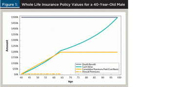
Figure 1 provides a visual representation for the case study numbers with a steady death benefit of $500,000 from age 40 to 100 (see the next section for the case study). The cash value grows to equal the value of the death benefit at age 100. Premiums are paid until age 65. By age 65, the cash value of $210,043 is higher than the $197,600 of cumulative premiums paid, but it took 20 years for positive returns net of insurance costs to manifest for the cash value. Whole life insurance is not designed to be a short-term strategy. After age 65, the cash value continues to grow despite the end of premiums, further reducing insurance costs, until the policy endows at age 100 when the cash value grows to match the death benefit. (Whole life policies are typically designed to endow at either age 100 or age 121.)
The Case Study
Consider a case study for a married couple, both age 40, with two children, and who are constructing a lifetime financial plan. The husband is seeking an additional amount of life insurance death benefit equal to $500,000. This, along with his other life insurance, will be sufficient to support his family in the event of his death prior to age 65.
He has $60,000 saved in his employer’s 401(k) plan, which is invested with an equity glide path strategy representative of a typical target date fund: 80 percent stocks to age 45; 65 percent stocks from age 45 to 54; 50 percent stocks from age 55 to 64; 40 percent stocks from age 65 to 74; and 30 percent stocks thereafter. He would like to plan for retirement at age 65.
This study investigated a portion of his assets to be saved in the future that is equivalent to 401(k) employee contribution limits in 2018 with assumed inflation adjustments: $18,500 can be saved each year until age 50, and then $24,500 thereafter until age 65. These contribution limits are inflation adjusted such that real savings are kept the same, but the nominal amounts increase.
Because life insurance premiums are fixed without inflation adjustments, the percentage of the savings directed to insurance decreases over time in real terms. The husband expects to be in a combined 32 percent marginal tax bracket both before and after retirement.
Investment returns. For investment returns, this study simulated stock returns with an equity premium above the fixed 3 percent bond yield. Inflation was fixed at 2 percent annually. This implied a fixed 1 percent real interest rate. The “risky” asset was based on large-cap stocks in the United States. Morningstar data revealed that the arithmetic average return on large-cap stocks for the period 1926 to 2017 was 12 percent with a standard deviation of 20 percent. This is 6 percent larger than the 6 percent average return earned historically by long-term U.S. government bonds. The subsequent analysis used this historical 6 percent equity risk premium with 20 percent standard deviation. Some readers may believe that the equity premium will be less in the future; reducing the equity premium would improve the relative performance of strategies using whole life insurance.
Monte Carlo simulations. To better understand the impacts of investment volatility on the upside and downside, Monte Carlo simulations were used to create a distribution of outcomes. The investment portfolio was modeled using 10,000 Monte Carlo simulations for stock returns based on these capital market expectations. As investments are held in tax-deferred accounts, there is no further tax drag to worry about. Investors earned the gross returns less the 1 percent fee, and portfolio distributions were taxed as income. The investment account values were expressed in post-tax terms assuming a 32 percent combined marginal tax rate.
Annuity pricing. Income annuities were priced with the same bond and mortality assumptions as described earlier with pricing life insurance. Income annuities were also priced with an annual 2 percent cost-of-living adjustment for payments to match the assumed inflation rate. For males, this corresponded to payout rates of 5.61 percent.
Tax treatment. A review of the tax principles used herein is also in order. Investments were made in the husband’s tax-deferred 401(k) plan, which was rolled over to an IRA at retirement. Life insurance premiums were paid with post-tax funds. No taxes were due on the death benefit, making it a post-tax number (a life insurance policy can also be arranged so that funds can be borrowed from the cash value without being taxed).
If an income annuity was purchased at retirement, this purchase was made with qualified retirement funds and annuity income was therefore fully taxable at income tax rates. Because the annuity was purchased in a qualified account, someone seeking to purchase an annuity with funds equivalent to the life insurance death benefit would need to inflate their purchase to account for the differing tax treatment. For example, a non-taxed death benefit of $500,000 is equivalent to $500,000 / (1 – 0.32), or $735,294, in a qualified account.
Term or whole life? The husband must decide whether to purchase a term life insurance policy to increase his existing coverage to meet his human capital replacement value for his family, or to otherwise purchase a whole life insurance policy that can serve his additional human capital replacement value need, as well as be integrated into his retirement income strategy. He will pay for life insurance premiums and the taxes to cover those premiums from his annual savings, and the remainder will go into his tax-deferred 401(k).
In all scenarios, the husband was directing at least enough to the 401(k) to satisfy the conditions for the highest possible company match, though this study did not specifically model any company match when simulating retirement income. More generally, the couple may also have other resources in retirement that were not analyzed. This study modeled the relevant features about how to best make the investment and insurance decisions for the described annual set-asides to meet life insurance needs and to obtain the most desirable retirement outcomes.
The term policy lasted for 25 years with a $500,000 death benefit and had an annual premium of $2,624. Taxes on the pre-tax income required to cover this premium were $1,235. After paying the term life premium and taxes, he contributed the remaining $14,641 to his 401(k).
The limited-pay whole life policy also carried a death benefit of $500,000. The annual premium was $7,904 until age 65. The policy accrued cash value that could serve as an additional spendable asset for the household. Taxes to cover the whole life premium were $3,720. With a whole life policy, the husband can contribute $6,876 to his 401(k) at age 40, with that value growing with the contribution limits.
Asset allocation. An important methodology issue for the case study relates to asset allocation. With a whole life policy, the cash value is a liquid asset contained outside the financial portfolio. It behaves like fixed income, though it is not exposed to interest rate risk (i.e. the accessible cash value does not decline when interest rates rise). Cash value is not precisely the same as holding bonds in an investment portfolio, as there is not a practical way to rebalance the portfolio between stocks and policy cash value. Nonetheless, the couple in the case study incorporated the cash value into their asset allocation decisions to maintain the overall proportion between stocks and bonds for household assets.
For example, if the target date fund called for a 50 percent stock allocation, then the actual stock allocation was 50 percent of the sum of the financial portfolio balance and the pre-tax value of life insurance cash value, divided by the portfolio balance. The maximum possible stock allocation for the financial portfolio was constrained to not exceed 100 percent.
Meeting a Legacy Goal During Retirement
This study first considered how the death benefit for life insurance provides a method to meet a legacy goal using risk pooling and tax advantages that are distinct from preserving investment assets for this purpose. This can allow the retiree to potentially enjoy a higher standard of living in retirement while ensuring sufficient assets have been earmarked to meet the legacy goal.
Table 1 compares the effectiveness of two strategies for meeting a legacy goal during retirement: (1) “buy term and invest the difference” in Scenario 1.1; and (2) using whole life insurance in Scenario 1.2. Values are expressed on an after-tax basis with a combined 32 percent tax rate applied to qualified plan distributions and legacy values. The cash value and death benefit from the whole life policy are not treated as taxable assets.
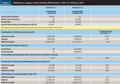
In getting more serious about their financial planning, the couple begins to think about their legacy goals for their children. They anchor onto their $500,000 current life insurance need and believe an appropriate legacy goal would be to leave their children this amount upon the husband’s passing, no matter the age. The couple would like to support the highest living standard possible while maintaining a 90 percent chance that a $500,000 after-tax legacy goal can continue to be met by age 100. The husband’s legacy goal for the investment assets inflates to $735,294 so that the after-tax amount of $500,000 can be achieved, assuming the adult children will also be in the 32 percent tax bracket for the inheritance received.
What is the most efficient way to meet this goal?
If the couple used whole life insurance, they could seek the highest spending rate for the remaining investment assets that maintains a 90 percent chance that the portfolio would not be depleted by age 100. They would not need the extra safety margin for investments, which would allow for a higher spending rate.
This is the trade-off that must be empirically tested: can the couple spend more or less in retirement when using whole life insurance after considering the offset between the higher insurance premiums and fewer 401(k) assets at retirement, but the ability to use a higher distribution rate from investments because there is no longer a need to maintain the safety margin with investments for legacy?
Table 1 provides these results. In Scenario 1.1, the couple purchases term insurance to provide a death benefit for human capital replacement until age 65. The remainder of their savings is invested in the husband’s 401(k) and they use this pot of investment assets to support their spending and post-retirement legacy goals. In Scenario 1.2, the couple maintains a whole life policy into retirement to cover legacy and invests the remainder in their 401(k) to cover retirement spending.
Because the whole life premiums are larger, the couple can expect to have less in their 401(k) at retirement. The difference ranges from 27 percent less at the 10th percentile of the distribution, to 4 percent less at the 90th percentile. Accumulations are generally less because less is invested. This is partially offset, however, through asset allocation in which the cash value is treated as a fixed income asset and so the 401(k) asset allocation can be made more aggressive in response. The more aggressive asset allocation particularly helps when markets perform well. Median 401(k) assets at retirement are $625,528 in Scenario 1.1 and $548,625 in Scenario 1.2.
Next, the table shows that the sustainable withdrawal rate is 1.73 percent in Scenario 1.1 and 2.87 percent in Scenario 1.2. They are different for two reasons. First, in Scenario 1.2, the asset allocation is more aggressive for investment assets because of the role played by cash value as a fixed income asset. Second, to meet the legacy goal, Scenario 1.1 requires a lower spending rate to support a 90 percent chance that remaining assets are not less than $500,000 after taxes at age 100 (instead of not being less than $0 in Scenario 1.2.). This means using a lower spending rate.
The higher distribution rate allows for more spending in Scenario 1.2, while meeting the legacy goal. In the median outcome, these assets can support 46 percent more inflation-adjusted spending throughout retirement than Scenario 1.1.
Finally, Table 1 shows legacy wealth at age 100. Recall that the couple sought a 90 percent chance to meet their legacy goal. Approximately $500,000 is left after taxes in both scenarios at the 10th percentile of the distribution.
For the remainder of the distribution, legacy wealth is less in Scenario 1.2. The couple must spend less in Scenario 1.1 to ensure that investments can support their stated legacy goal. If they do not experience the bad market environment, Scenario 1.1 supports a larger legacy than intended at the cost of not enjoying as high of lifestyle as otherwise possible.
The couple maintains extra reserves for their investment portfolio to ensure legacy, which means they spend less and may end up leaving behind even more. In Scenario 1.2, pooling risk through life insurance allows them to instead enjoy a higher standard of living throughout retirement while still meeting their stated legacy goal. At the median, they enjoy spending 46 percent more throughout retirement and at age 100 face a legacy that is 23 percent less than in Scenario 1.1 (however, it is $451,000 more than their targeted goal).
Because investments are used as the source of legacy in Scenario 1.1, it becomes necessary to remain extra cautious about retirement spending to maintain the desired safety margin for investments.
Including an Income Annuity in the Retirement Plan
The second notion this study explored is how a permanent death benefit supported through whole life insurance could be integrated into a retirement income plan by helping the retiree justify the decision to buy an income annuity. In this case study, the hypothetical retiree purchases a life-only single life annuity that offers the most mortality credits and therefore the highest payout rate to the owner. From a behavioral finance standpoint, the retiree can feel comfortable buying an income annuity because the life insurance death benefit will return the amount spent on the annuity premium to the household at the time of death.
Table 2 adds two additional scenarios for this investigation. Scenario 2.1 uses the same “buy term and invest the difference” strategy as Scenario 1.1, but now there is no specific legacy goal to be funded. The couple may spend more aggressively from their 401(k) assets in retirement. Upon reaching age 65 in 25 years, the couple will consider whether a single-premium immediate annuity (SPIA) might be a worthwhile addition to their retirement income plan.
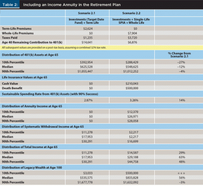
Scenario 2.2 integrates investments with a whole life insurance policy and with a single life income annuity purchased at retirement. With a single life annuity, the death benefit will replace this asset for the household when the annuity payments stop. A male life-only income annuity offers the highest payout rate because the buyer offers the most mortality credits to the risk pool since survival odds are the lowest. The income annuity includes a 2 percent annual cost-of-living adjustment that matches the assumed inflation rate.
With the accumulated investment assets, all retirement income in Scenario 2.1 is generated with a systematic withdrawal strategy. The couple uses the highest withdrawal rate possible that keeps investments above $0 by age 100 with a 90 percent probability. In Scenario 2.1, spending from these assets falls to $0 once the portfolio balance depletes.
Next, in Scenario 2.2 the couple uses a whole life insurance policy and purchases a male life-only income annuity at age 65 with an amount of assets equivalent to the pre-tax value of the death benefit ($735,294). In simulations where the investment balance has not grown sufficiently to leave at least $100,000 remaining after the annuity is purchased (to provide the couple with a pool of liquid assets to support contingency expenses), then the couple only annuitizes the amount that leaves $100,000 of liquid investable assets (on a pre-tax basis) after the annuity is purchased. After annuitization, the remaining portfolio balance will be used for retirement spending, using a systematic withdrawal strategy that maintains a 90 percent probability that the account remains above $0 by age 100. Portfolio depletion is less drastic in this case, with the inflation-adjusted annuity income continuing for life.
Table 2 outlines the retirement outcomes. Scenario 2.1 presents the strategy for buying term insurance and investing the difference in a target date fund. In after-tax terms at retirement, the wealth accumulation ranges from $392,954 at the 10th percentile to $1.06 million at the 90th percentile, with a median outcome of $625,528. With the capital market expectations, expenses, and asset allocation decisions, the sustainable spending rate that supports a 90 percent chance that assets remain at age 100 is 2.87 percent. This spending rate supports an after-tax, inflation-adjusted retirement income ranging from $11,278 at the 10th percentile to $30,291 at the 90th percentile, with a median of $17,953.
As for legacy wealth at age 100, it ranges from $3,033 at the 10th percentile to $1.68 million at the 90th percentile, with a median amount of $535,575. Legacy wealth consists of the after-tax value of any remaining financial assets in the investment portfolio and any life insurance death benefit. With Scenario 2.1, there is no annuitization or death benefit. Investment assets are the only resource to support spending and legacy in retirement.
Scenario 2.2 integrates investments with whole life insurance and income annuities. With partial annuitization through a single-life SPIA with a 5.61 percent payout for an amount equal to the death benefit of the whole life policy at age 65, inflation-adjusted annuity income is $28,058 after taxes are paid. It is less at the 10th and 50th percentiles because a smaller amount could be annuitized to preserve $100,000 of investment assets for liquidity. Annuity income grows with the same 2 percent cost-of-living adjustment to match the assumed overall inflation rate.
The 3.26 percent withdrawal strategy (driven by the more aggressive asset allocation that accounts for the cash value and annuities) is then applied to any remaining investment assets, generating additional income. More aggressive allocations tend to support a higher sustainable spending rate with the same objective of maintaining a 90 percent chance that investment assets are not depleted at age 100. Total retirement income at age 65 ranges from $14,587 to $44,758, with a median of $29,188.
As for legacy wealth at age 100, Scenario 2.2 maintains the death benefit of $500,000 after taxes, which is still available despite investments depleting at the 10th percentile. At the median, Scenario 2.2 supports legacy wealth of $833,828, which is 56 percent larger than in Scenario 2.1. Of this, $500,000 is the death benefit and the other $333,828 is the remaining portfolio balance after taxes. At the 90th percentile, investments have performed very well; legacy wealth is 3 percent less than Scenario 2.1, however it is still $1.63 million.
Generally, the integrated approach provides more legacy wealth while supporting more retirement income. At the median, Scenario 2.2 provides 63 percent more lifetime spending and 56 percent more legacy than Scenario 2.1.
Cash Value as a Volatility Buffer
The third scenario this analysis explored is that whole life insurance cash value may serve as a volatility buffer to help manage sequence of returns risk. Cash value does not experience downside risk for capital losses in the face of rising interest rates. It is guaranteed to grow and can provide a temporary resource to supplement retirement spending rather than being forced to sell portfolio assets at a loss during poor market environments.
Table 3 provides a new volatility buffer scenario to compare with “buy term and invest the difference.” In Scenario 3.2, investments are combined with whole life insurance and the cash value is available to be used entirely as a volatility buffer to help support the portfolio and maximize retirement spending. Once partial surrenders are used to obtain cash value up to the cost basis, policy loans are taken with the remainder of the cash value serving as collateral to avoid taxes on these distributions. A conservative loan interest rate of 8 percent is used to grow the loan balance.
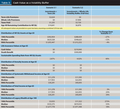
The whole life policy is assumed to use non-direct recognition; there is no adjustment to the growth for the cash value that has been used as collateral for loans. Legacy values at age 100 reflect any remaining investment assets along with the remaining net life insurance death benefit after offsetting cash value surrenders and any loans plus accumulated interest.
One must be careful that interest on the loan balance does not push the loan balance over the limit of the available cash value. Such an outcome should be avoided so taxes are not triggered on all life insurance policy gains in one tax year. The maximum amount that can be taken from the cash value in any year is the amount that would not grow with interest (at 8 percent) to exceed the slower growing cash value by age 100 (with an additional $5,000 buffer of protection so that the net cash value does not fall entirely to $0). This process ensures that the loan balance growth stays below the cash value, protecting the policy from “blowing up.” In practice, this outcome can be avoided by monitoring the policy and paying down the loan balance if it is approaching the total cash value limit.
The cash value can be used as a buffer to help manage sequence of returns risk. Maintaining fixed distributions from investments in retirement increases exposure to sequence risk by requiring a higher withdrawal rate from remaining assets when their value declines. Temporarily drawing from the whole life cash value could potentially mitigate this aspect of sequence risk by reducing the need to take portfolio withdrawals at inopportune times. Whether or not this strategy will work becomes an empirical question to be tested.
Aggressively using the volatility buffer to support more retirement spending involves making a conscious decision to focus on increasing spending at the potential cost of legacy. The investments-only strategy forces spending to be conservative, feeding instead into a larger legacy, because of its inefficient approach for managing longevity and market risk. Nonetheless, limited use of the volatility buffer may not reduce legacy. Using the volatility buffer reduces the net death benefit, but the investment portfolio may ultimately grow by more than the reduction to the death benefit, potentially leaving a larger net legacy. This outcome can result from the peculiarities of sequence risk and the ability to avoid selling portfolio assets at a loss.
Life insurance also receives tax benefits, and the distribution from the cash values can be less because taxes are not paid on the proceeds. The idea is to spend from the cash value in years after a market downturn, and spend from the investment portfolio in years after positive market returns.
In Table 3, Scenario 3.1 is the classic “buy term and invest the difference” strategy. It is repeated in Table 3 to serve as a baseline for comparison. Because the cash value provides an additional base of assets to replace some portfolio distributions as well as a fixed income resource that allows the stock allocation in the investment portfolio to be increased, the initial withdrawal rate for investments increases from 2.87 percent to 4.02 percent in Scenario 3.2 while maintaining a 90 percent chance that investment assets remain at age 100.
Inflation-adjusted spending in retirement increases between 3 percent and 34 percent across the distribution. The median increase in distribution of total income at age 65 is 23 percent. Meanwhile, legacy assets are also better supported in Scenario 3.2 with the volatility buffer helping to manage sequence risk for the investment portfolio. At the median, legacy assets are 53 percent larger at age 100.
Across the distribution of outcomes, spending and legacy are larger in Scenario 3.2 than in Scenario 3.1. Whole life insurance used as a cash value volatility buffer appears to beat “buy term and invest the difference” for a lifetime financial plan initiated by the couple, both age 40, in this scenario.
Conclusion
This analysis revealed that advisers should not blindly follow the common notion of “buy term and invest the difference” when seeking to create the most efficient lifetime financial plans for their clients. In some situations, the power of risk pooling in a lifetime financial plan should not be overlooked.
Endnotes
- See, “Can an Investor Reduce their Overall Portfolio Risk by Allocating from Fixed Income to a Whole Life Insurance Policy?” by Morningstar Investment Management LLC, which used data provided by New York Life that was not independently verified by Morningstar for accuracy.
- See “Life Tables for the United States Social Security Area 1900–2100,” at ssa.gov/oact/NOTES/as116/as116LOT.html.
References
Babbel, David F., and Oliver D. Hahl. 2015. “Buy Term and Invest the Difference Revisited.” Journal of Financial Service Professionals 69 (3): 92–103.
Fechtel, R. Brian. 2012. “Bringing Real Clarity and Understanding of Cash-Value Life Insurance to the Marketplace.” Journal of Financial Planning 25 (9): 50–59.
Pfau, Wade D. 2015. “Optimizing Retirement Income by Combining Actuarial Science and Investments.” Retirement Management Journal 5 (2): 15–32.
Sacks, Barry H., and Stephen R. Sacks. 2012. “Reversing the Conventional Wisdom: Using Home Equity to Supplement Retirement Income.” Journal of Financial Planning 25 (2): 43–52.
Smith, Michael L. 1982. “The Life Insurance Policy as an Options Package.” The Journal of Risk and Insurance 49 (4): 583–601.
Teitelbaum, Mark A. 2014. “Smooth Sailing on Uncertain Waters: Using Life Insurance to Steady the Ups and Downs of Retirement Assets.” The Wealth Channel Magazine (Fall): 25–30.
Citation
Pfau, Wade D. 2019. “Investigating the Role of Whole Life Insurance in a Lifetime Financial Plan.” Journal of Financial Planning 32 (2): 44–53.