Journal of Financial Planning: February 2016
Kyoung Tae Kim, Ph.D., is an assistant professor in the Department of Consumer Sciences at the University of Alabama. He received a Ph.D. in consumer sciences from The Ohio State University.
Sherman D. Hanna, Ph.D., is a professor in the Human Sciences Department at The Ohio State University. He is the program director of the CFP Board-registered undergraduate financial planning program.
Executive Summary
- The Great Recession caused financial problems for many households in terms of unemployment, business losses, and decreases in real estate values; overall, the broadly based decreases in stock indexes impacted households in all areas of the U.S.
- The decreases in stock market indexes between 2007 and 2009 had substantial impacts on the wealth of only a small proportion of working households, with a mean potential loss in wealth due to stock market decreases of only 1.3 percent.
- The relative impact of the stock market declines was highest for the oldest working households, but the mean potential loss in wealth for that group was 1.9 percent; only 5 percent of households in that age range had a potential loss of 8 percent or more of wealth.
- By framing the potential wealth loss from a severe stock market decrease as a percent of wealth including human wealth, financial planners can add another perspective to assist clients in thinking rationally about portfolio choices.
The Great Recession began in December 2007 and officially ended in June 20091, although high unemployment, substantial drops in housing prices, and high foreclosure rates continued for years after 2009. The impact on the stock market was also severe. For instance, the Dow Jones Industrial Average reached a peak before the Great Recession of 14,088 on October 1, 2007 and decreased to 6,547 by March 9, 2009, a decrease of 54 percent. Bricker, Bucks, Kennickell, Mach, and Moore (2011) reported that the mean net worth of U.S. households fell from $595,000 in 2007 to $481,000 in 2009.
U.S. workers have become more responsible for their own retirement savings over the past several decades. This is the result of defined benefit pension plans being replaced by defined contribution pension plans. Defined contribution plans require participants to manage asset allocation choices. The ability to manage these portfolios efficiently can have an important impact on financial well-being in retirement (Browning and Finke 2015). However, many investors are prone to make financial mistakes due to their lack of market experience, which results from being young and a decrease in cognitive ability for some older investors.
Many investors have fears about investment decisions (Budgar 2011), anchoring biases (Astorino 2015), and misperceptions of risk (Carpenter 2013), especially during periods of economic recession. One role for financial planners is to communicate with their clients to overcome market fears. Vanguard quantified the value of wealth management advice (gamma) at approximately 3 percent, which is related to rebalancing, behavioral coaching, access to research, strategy development, and income source selection (Kinniry, Jaconetti, DiJoseph, and Zilbering 2014). For instance, a financial planner could inform a client about the history of stock market recoveries after bear markets (Leonard 2009). This information could then help the client alter behavioral intentions.
Financial planners could also help clients identify the share of equity investments in the total wealth of the household. For instance, a young worker might have 100 percent of financial investments in stock funds, but those investments might represent a small fraction of total future lifetime earnings, or human wealth. Chen, Ibbotson, Milevsky, and Zhu (2006) discussed the importance of considering portfolio allocations in the context of the total wealth of a household, including human wealth. They noted that human capital (human wealth) is typically worth much more than financial capital for young investors, so the optimal allocation to risk-free financial investments may be initially very low. They also discussed the role of the volatility of human capital in optimal allocation of financial investments, as workers who have volatile earnings should consider a lower level of volatility in the financial portfolio.
Research Objective
This study had the objective of estimating the impact of the stock market decreases during the 2007–2009 period on the total wealth of working households. By providing a human wealth-based framework of lifetime wealth shock, this study can help financial planners provide their clients better perspectives to prepare for future stock market declines.
Using the 2007–2009 Survey of Consumer Finances panel dataset, this study also estimated each household’s human wealth in addition to other forms of wealth. The study was limited to households before retirement, when presumably the focus is on accumulating investments. Only households in which the head of the household was employed full-time were included, as there may be more uncertainty in projecting the future earnings of other households.
This research provides important insights for financial planners regarding the rational assessment of portfolio losses of their clients. Put in the context of total wealth, including human wealth, even the severe stock market crash in the 2007–2009 period resulted in small potential losses relative to total wealth for all but a small proportion of households.
Data and Sample Selection
The Board of Governors of the Federal Reserve System has released the Survey of Consumer Finances (SCF) triennially since 1983. The SCF is designed to provide very detailed information on all aspects of households’ finances, including the types and amounts of assets, liabilities, and income. The regular SCF is a cross-sectional dataset, but because of the Great Recession, the 2009 SCF panel dataset was collected, interviewing most of the households interviewed in the 2007 survey (Bricker et al. 2011). The 2007 SCF was the first wave based on the 2007 SCF cross-sectional dataset, with interviewing starting in May 2007, and almost all of the interviews were completed by the end of 2007, although a small number were conducted in the first three months of 2008 (Kennickell 2008). The 2009 re-interviews started July 28, 2009 and almost all were completed by the end of 2009 (Kennickell 2010).
The main analyses in this study were restricted to households whose heads were employed full time and who were age 30 to 70 in the first survey wave. The total sample size of the 2007–2009 SCF panel dataset was 3,857, and 2,294 households met the sample criteria for this research. For a more robust analysis, imputed cases of expected retirement ages and working status were excluded. Additionally, the 273 households that changed heads between 2007 and 2009 were excluded, because this study focused on financial decisions made by the household head. The final sample size was 2,021.
Measurement of Financial Wealth Shock
In addition to substantial losses in housing wealth during the 2007 recession, many households experienced significant losses in their financial wealth following the stock market crash in October 2008. The Great Recession caused substantial losses in several components of household balance sheets, including stock assets in retirement funds, the value of personal residences, the value of business assets owned by households and not in publicly traded companies, and the value of real estate assets other than one’s personal residence.
Investments other than stock assets are substantial components of the balance sheet for some households (Hanna, Wang, and Yuh 2010). However, other major types of risky investments have idiosyncratic patterns of gains and losses, with, for instance, substantial drops in real estate values in some parts of the U.S., but small drops in other parts. Some owners of privately held business assets might have had substantial decreases, while others had gains. Therefore, following previous research, this research considered the financial wealth shock limited to the estimated potential decrease in stock assets from the time of the 2007 interview to the time of the 2009 interview. Rather than use actual decreases in equity balances, the potential loss was calculated for each household. Additional details on the estimation can be found in Kim (2014).
Recent studies on financial wealth shocks used the S&P 500 Index to capture possible fluctuations in stock market value (Coile and Levine 2011; Goda, Shoven, and Slavov 2011; Schwandt 2011). For example, Coile and Levine used changes in the S&P 500 for one year, five years, and 10 years, respectively, because of the unclear time frame in which individuals respond to market fluctuations. Similarly, Goda et al. used the annual percent growth rate in the S&P 500 during the 12 months prior to the interview date. Schwandt used a more comprehensive measurement of wealth shock. He constructed stock market-induced wealth shocks as the product of the lagged fraction of total wealth held in stocks with stock market percentage change. The total wealth was the sum of current wealth holdings and discounted expected future pension income. The percentage change in the S&P 500 was used to capture stock market fluctuation.
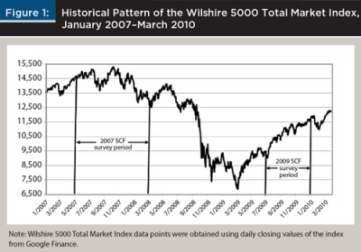
In this research, the potential effect of the Great Recession on total wealth was estimated using Schwandt’s (2011) constructed wealth shock measurement. His measurement was applied in the current study to the SCF panel dataset. Information about individual respondents’ survey date was not available in the SCF public dataset, but, the SCF includes for each household the level of an alternative stock market index—the Wilshire 5000 Total Market Index—on the day of the 2007 SCF interview and the day of the 2009 SCF interview. The Wilshire 5000 is based on more than 5,000 capitalization-weighted security prices.
Figure 1 presents the level of the Wilshire 5000 based on daily closing values and the timing of each SCF survey wave. Note that households were interviewed for the 2007 survey during a time when the Wilshire 5000 ranged from 12,508 to 15,294. During the re-interview period, the index ranged from 10,026 to 11,678.
Projection of Total Wealth
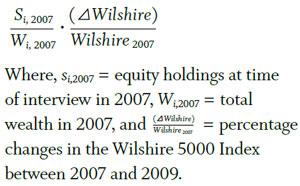
Similar to total wealth discussed by Schwandt (2011), this study used total wealth, defined as the sum of current net worth and estimated human wealth. As a major component of total wealth, human wealth was projected as the present value of future flows of non-investment income, following methods presented by Gutter (2000) and Wang (1997). The constructed financial wealth shock was defined as follows:
Net worth. The SCF dataset provides comprehensive measures of household net worth computed by subtracting the amount of debts from the amount of assets. Household assets include financial assets, such as checking and savings accounts and other financial investments, and non-financial assets, such as housing, vehicles, other real estate, and businesses. All types of household debts are included.
Human wealth. Human wealth included the present value of future salaries, wages, and self-employment earnings, as well as the present value of anticipated pensions, including Social Security (see Gutter 2000 and Wang 1997). In order to calculate human wealth, two important assumptions about the working horizon and the retirement period were made. The expected retirement age reported by respondents in 2007 was used to set the number of working years until retirement. The method that Gutter (2000) used for the remaining life expectancies at the expected retirement age was used in this research.
The number of years before the expected retirement age was used to calculate the present value of future salaries. The SCF provides the pre-tax amount of earning on each respondent’s jobs and the jobs of a spouse/partner if there was one. For couple households, the present value amount was calculated based on the earnings of both spouses/partners. Gutter (2000) assumed earnings growth based on a respondent’s expectation for future income, setting a real growth rate of 3 percent households, expecting income to increase faster than prices in the following year and a zero percent growth for other households. However, to be conservative, in this research, a zero rate of inflation-adjusted increases was used in all earnings projections.
The SCF also provides information about business income. For households receiving income from businesses, this research followed a conservative assumption made by Gutter (2000) and Wang (1997) that business income will not be available once the household retires (note that the value of a business was counted in net worth). To calculate the present value of the labor income stream, a relatively high discount rate was applied, because pre-retirement income was uncertain. In this study, the historical inflation-adjusted large stock return was used as a discount rate for labor force income (Ibbotson Associates 2008). Lastly, this study only included households with full-time working heads, so there were no households with zero income. If a worker expected to work part time after retirement, it was assumed that income would be 30 percent of the full-time wage.
The projection method for Social Security retirement benefits followed the estimation method reported by Gutter (2000) and Wang (1997). All households with positive earnings were assumed to be eligible for Social Security retirement benefits. Social Security benefits were calculated based on each worker’s year of birth, with current wage used as a proxy for a worker’s earnings averaged over the working lifetime. Then, the Primary Insurance Amount (PIA) was calculated at an individual worker’s full retirement age, using the method recommended by Yuh, Hanna, and Montalto (1998), Montalto, Yuh, and Hanna (2000), and Kim, Hanna, and Chen (2014).
The projected Social Security pension was calculated based on each respondent’s expected retirement age, using assumptions made by the researchers cited. If a household head reported an expected retirement age less than 62, Social Security benefits were assumed to begin at age 62, and there would be no wages between the expected retirement age and age 62. Future Social Security benefits were discounted by using the historical inflation-adjusted rate of return on intermediate government bonds from 1926–2007 of 2.6 percent (Ibbotson Associates 2008).
The SCF provides information about defined benefit pension plans for each respondent and spouse. Specifically, the amount of the benefit and the anticipated age to receive benefits from current or past employers. To calculate the future retirement benefit stream, the years of defined pension benefits were determined between the expected benefit age and death age as estimated by life expectancy. As with the Social Security benefit projection, benefits were discounted by using the historical inflation-adjusted rate of return on intermediate government bonds (Ibbotson Associates 2008).
The present values of the Social Security and defined pension benefits were defined as follows:
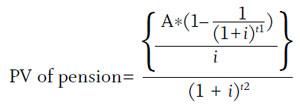
Where, A was the amount of annual Social Security or defined benefit pension projected at retirement; i was the discount factor (2.6 percent); t1 was the number of years the person will receive benefits during retirement; and t2 was the number of years prior to receipt of benefits from the current period.
The discount rate for labor force income was 8.5 percent, which was the inflation-adjusted rate of return on large stocks, based on historical returns from 1926–2007 (Ibbotson Associates 2008). The rationale for using the 8.5 percent discount rate was to discount for the uncertainty of future income, due to factors such as unemployment, disability, and death of a household member. The future stream of labor force income was less certain than income received during retirement, such as Social Security and defined benefit pension income.
Results
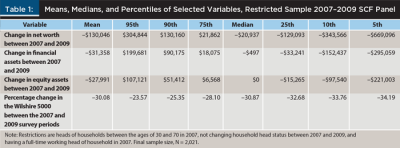
Table 1 shows the distribution of changes in the value of household net worth, financial assets, and equity assets over the 2007–2009 period. The last row of Table 1 shows the distribution of percent changes in the Wilshire 5000, which was an important driver of the potential wealth shock measure. (As noted previously, households were interviewed on different dates in 2007 and in 2009, resulting in a range of percent changes in the index.) The mean net worth change was –$130,046. The mean financial assets change was –$31,358. The mean equity assets change was –$27,991. The top 5 percent in terms of decreases in equity assets had a decrease of at least $221,003, while 5 percent of households had an increase of $107,121 or more (95th percentile).
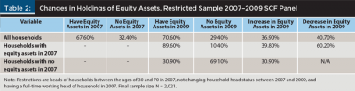
As shown in Table 2, for all households in the analytic sample, 41 percent had a decrease in equity assets, although 32 percent of the households had no equity assets in 2007. Of the households with equity assets in 2007, 10 percent had no equity assets in 2009. Of the households with no equity assets in 2007, 31 percent had equity assets in 2009. Of the households with equity assets in 2007, 40 percent had an increase in equity assets.
The value of equity assets might have changed for a household over this period for a variety of reasons. A household might have sold all of its stock assets just after being interviewed in 2007, and therefore would have exhibited a decrease in equity assets. It is also possible that a worker might have had no equity assets at the time of the interview in 2007, but might have started participating in an employer retirement plan invested in stock funds, and with employee plus employer contributions, might have had a substantial increase in equity assets. It was not possible to completely identify in the SCF dataset all possible reasons for changes in equity assets. It was also not possible to identify specific stocks or funds owned by households. Therefore, in this research, a measure similar to Schwandt’s (2011) potential equity asset change was used.
For each household in the SCF panel, the percent changes in the Wilshire 5000 depended on the interview date in 2007 and in 2009. Table 1 shows the distribution of percent changes. The large decreases (the top 5 percent had –34.19 percent or worse) were for households interviewed near the highest market level during the 2007 period and the lowest level in the 2009 period, while the smallest decreases (5 percent had a decrease of –23.57 percent or better) were interviewed near the end of both interview periods.
Table 3 shows total wealth, mean equity holdings as a percentage of total wealth, and mean and median potential wealth shock and equity holdings for all households and for each quartile of net worth in 2007. The potential financial wealth shock as a percent of total wealth was calculated for each household based on its level of equity assets at the time of the interview in 2007 and the percent decrease in the Wilshire 5000 between the day of the 2007 interview and the day of the 2009 interview. Therefore, the potential wealth shock indicates what loss each household could have had in its equity holdings at the time of the 2007 interview, assuming no reallocation. Given the recovery in stock indexes since 2009, an investor who simply held stocks and stock funds would have more than recovered the losses, but this measure gives an indication of a worst case loss (for example, an investor who sold all stock holdings near the bottom of the market).
The patterns of financial wealth shocks as a percent of wealth by net worth quartile indicate that the losses were greater for households with a higher net worth than for those in the lower quartiles of net worth. Means tests based on the repeated-imputation inference (RII) technique were used to examine differences of wealth shock between net worth quartiles. The mean value of potential wealth shock, as a percent of wealth, was the highest in the top quartile (–3.1 percent of wealth) and lowest in the bottom quartile of net worth (–0.1 percent of wealth.) Results show significant differences in mean wealth shock between net worth quartiles. Many of the households in the lowest net worth quartile had no stock assets, so they were not affected by decreases in stock prices.
Table 4 shows total wealth, mean equity holdings as a percent of total wealth, and mean and median potential wealth shock and equity holdings for each quartile of age of head of household in 2007. The quartiles of age of household head in 2007 were 30–37, 38–45, 46–53, and 54–70. Total wealth was the highest ($2,258,505) for households aged 54–70, while it was lowest ($1,132,292) for the youngest group, those aged 30–37. The youngest group had a mean potential wealth shock of –0.6 percent of total wealth, while the wealth shock of the oldest group had a mean value of –1.9 percent. Means tests showed that there were significant differences in mean wealth shock between age groups.
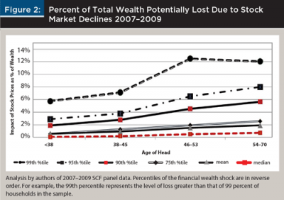
Figure 2 shows the distribution of wealth shock for each quartile of the age of head of household. The potential wealth loss for the median and mean financial wealth shock increased with age of the head of household, but only small proportions of households had losses over 5 percent of wealth. At the 95th percentile, the wealth shock ranged from –3 percent for those under 38 year of age to –8 percent for those aged 54 to 70. The potential wealth shock was very small for all age groups, except at the 99th percentile.
Discussion
This study investigated the impact of the 2008–2009 stock market crash on the potential wealth loss of U.S. workers, using the 2007–2009 SCF panel dataset. This analysis of stock market shock differs from previous studies by using changes in the Wilshire 5000 for each household between 2007 and 2009, and considering the potential loss in equity assets as a percent of total wealth, including human wealth. The potential loss was estimated based on the percentage loss in equity assets as of the time of the household’s interview for the 2007 survey, and assuming at the time of the 2009 interview, the household sold all of its equity assets and the percentage decrease in value was the same as the percent loss in the Wilshire 5000.
The mean proportion of household wealth in equity assets in 2007 was only 4.2 percent. The mean potential loss in wealth from the decrease in the Wilshire 5000 during the survey period was only 1.3 percent. A small proportion of working households had a substantial potential loss. For instance, among households with a household head aged 54–70, only 5 percent had a potential loss of 8 percent or more of wealth. The relative impact of the stock market crash was less for households in the youngest age group compared to households in the oldest age group. This was the result of equity investments representing a much smaller proportion of total wealth for the younger households.
Overall, the results show that although households faced financial distress because of the stock market crash of 2008–2009, the impact of market declines on total wealth was limited in scope. While many fearful clients may be no more comforted by these results than Leonard’s (2009) findings that diversified portfolios typically fully recover from bear markets in three to five years, some may find this additional perspective useful.
For financial planners working with younger investors, a focus on the role of the human capital component of total wealth may help make those clients more comfortable with the volatility of a higher return investment portfolio. However, the volatility of human capital should be considered, as noted by Chen et al. (2006). For households nearing retirement, the willingness and ability to delay retirement (Blanchett 2013) could affect the portfolio allocation, as even the somewhat high potential wealth shock for the top 1 percent of households in the oldest age group, 12 percent (see Figure 2) could have been lessened by not selling all equity investments near the bottom of the crash.
This research did not address the impact of the stock market crash on retired households. Portfolio advice for retired households is complicated by withdrawal strategies (see Pfau and Kitces 2014) and whether inflation-adjusted spending needs to be maintained. As Delorme (2015) noted, a plan for constant inflation-adjusted retirement spending might not be safe, so the ability of a household about to retire to adjust retirement spending will affect the severity of a stock market crash on household wealth. Applying the approach presented in this paper to situations faced by retirees is worthy of additional research.
Endnote
- According to the National Bureau of Economic Research Business Cycle Dating Committee report, “Determination of the June 2009 Trough in Economic Activity,” dated September 20, 2010. See www.nber.org/cycles/sept2010.pdf.
References
Astorino, Francis. 2015. “How Anchoring Biases Influence Clients’ Financial Behavior.” Journal of Financial Planning 28 (6): 20–21.
Blanchett, David M. 2013. “The ABCDs of Retirement Success.” Journal of Financial Planning 26 (5): 38–45.
Bricker, Jesse, Brian Bucks, Arthur Kennickell, Traci Mach, and Kevin Moore. 2011. “Surveying the Aftermath of the Storm: Changes in Family Finances from 2007 to 2009.” Federal Reserve Working Paper, 2011–2017.
Browning, Chris, and Michael Finke. 2015. “Cognitive Ability and the Stock Reallocations of Retirees During the Great Recession.” Journal of Consumer Affairs 49 (2): 356–375.
Budgar, Laurie. 2011. “Communicating to Overcome Client Market Fears.” Journal of Financial Planning 24 (10): 20–25.
Carpenter, Michael. 2013. “Help Investors Make Better Risk/Reward Decisions.” Journal of Financial Planning 26 (10): 22–23.
Chen, Peng, Roger G. Ibbotson, Moshe A. Milevsky, and Kevin X. Zhu. 2006. “Human Capital, Asset Allocation, and Life Insurance.” Financial Analysts Journal 62 (1): 97–109.
Coile, Courtney, and Phillip B Levine. 2011. “The Market Crash and Mass Layoffs: How the Current Economic Crisis May Affect Retirement.” The B.E. Journal of Economic Analysis & Policy 11 (1): Contributions Article 22.
Delorme, Luke. 2015. “A Blueprint for Retirement Spending.” Journal of Financial Planning 28 (9): 40–50.
Goda, Gopi S., John B. Shoven, and Sita N. Slavov. 2011. “What Explains Changes in Retirement Plans during the Great Recession?” American Economic Review 101 (3): 29–34.
Gutter, Michael S. 2000. “Human Wealth and Investment Ownership.” Financial Counseling and Planning 11 (2): 9–20.
Hanna, Sherman D., Cong Wang, and Yoonkyung Yuh. 2010. “Racial/Ethnic Differences in High Return Investment Ownership: A Decomposition Analysis.” Journal of Financial Counseling and Planning 21 (2): 44–59.
Ibbotson Associates. 2008. Stocks, Bonds, Bills, and Inflation Yearbook. Chicago, IL: Ibbotson Associates.
Kennickell, Arthur B. 2008. “The Bitter End? The Close of the 2007 SCF Field Period.” Federal Reserve Working Paper.
Kennickell, Arthur B. 2010. “Try, Try Again: Response and Nonresponse in the 2009 SCF Panel.” Federal Reserve paper prepared for the 2010 Joint Statistical Meetings, Vancouver, Canada.
Kim, Kyoung T. 2014. “The Impact of the 2007 Recession on the Retirement Decisions of U.S. Households: Evidence from the 2007–2009 Survey of Consumer Finances Panel Dataset.” Unpublished dissertation, The Ohio State University.
Kim, Kyoung T., Sherman D. Hanna, and Samuel C. Chen. 2014. “Consideration of Retirement Income Stages in Planning for Retirement,” Journal of Personal Finance 13 (1): 52–64.
Kinniry, Francis M., Colleen M. Jaconetti, Michael A. DiJoseph, and Yan Zilbering. 2014. “Putting a Value on Your Value: Quantifying Vanguard Advisor’s Alpha.” Vanguard research paper.
Leonard, Scott A. 2009. “U.S. Equity Returns after Major Market Crashes.” Journal of Financial Planning 29 (10): 84–94.
Montalto, Catherine P., Yoonkyung Yuh, and Sherman D. Hanna. 2000. “Determinants of Planned Retirement Age.” Financial Services Review 9(1): 1–15.
Pfau, Wade D., and Michael E. Kitces. 2014. “Reducing Retirement Risk with a Rising Equity Glide Path.” Journal of Financial Planning 27 (1): 38–45.
Schwandt, Hannes. 2011. “Wealth Shocks and Health Outcomes: Evidence from Stock Market Fluctuations.” SSRN working paper.
Wang, Hui. 1997. “An Empirical Analysis of Household Asset Allocation Based on a Rational Expectations Model.” Unpublished dissertation, The Ohio State University.
Yuh, Yoonkyung, Sherman D. Hanna, and Catherine P. Montalto. 1998. “Mean and Pessimistic Projections of Retirement Adequacy.” Financial Services Review 9 (3): 175–193.
Citation
Kim, Kyoung Tae, and Sherman Hanna. 2016. “The Impact of the 2008–2009 Stock Market Crash on the Wealth of U.S. Households.” Journal of Financial Planning 29 (2): 54–60.