Journal of Financial Planning: February 2013
Executive Summary
- This paper outlines a different way to think about building a retirement income strategy that dramatically moves away from the concepts of safe withdrawal rates and failure rates. The focus is how to best meet two competing financial objectives for retirement: satisfying spending goals and preserving financial assets.
- Much of the current failure-rate framework fails to consider the retiree’s entire balance sheet of income-generating assets, such as Social Security and immediate annuities; ignores lost potential enjoyment from spending more early in retirement; and ignores the magnitude and severity of “failure.”
- The process described in this paper focuses on allocating assets between a portfolio of stocks and bonds, inflation-adjusted and fixed single-premium immediate annuities (SPIAs), and variable annuities with guaranteed living benefit riders (VA/GLWBs).
- This process incorporates unique client circumstances, bases asset return assumptions on current market conditions, uses a consistent fee structure for a fair comparison between income tools, operationalizes the concept of diminishing returns from spending by incorporating a minimum-needs threshold and a lifestyle spending goal, and uses survival probabilities to calculate outcomes. It also incorporates client preferences to balance the competing financial objectives for the final choice among the collection of allocations that define the efficient frontier for retirement income.
- The paper presents results for a 65-year-old couple whose lifestyle needs require a 4 percent inflation-adjusted withdrawal rate from retirement-date financial assets. Their efficient frontier generally consists of combinations of stocks and fixed SPIAs. Perhaps surprisingly, bonds, inflation-adjusted SPIAs, and VA/GLWBs are not part of the efficient frontier in the couple’s optimal retirement income portfolio.
Wade D. Pfau, Ph.D., CFA, is an incoming professor of retirement income at The American College, and winner of the Journal’s 2011 Montgomery-Warschauer Award. He holds a doctorate in economics from Princeton University, and he blogs frequently on retirement income research at wpfau.blogspot.com. See his Google+ profile for contact information, or email him at wadepfau@gmail.com.
William Bengen’s seminal 1994 article on sustainable withdrawal rates in the Journal of Financial Planning provided a much needed reality check on popular retirement discourse by demonstrating how the sequence of returns risk causes the sustainable withdrawal rate from a portfolio of volatile assets to fall below the average return to those assets.
Bengen described the SAFEMAX, which he defined as the sustainable withdrawal rate from the worst-case scenario in history. It was closer to 4 percent than to numbers like 7 percent bandied about in the media at that time. Bengen’s research answered an important question about sustainable spending rates. Several years later, Cooley, Hubbard, and Walz (1998) published a study popularly known as the Trinity study. It introduced a small but significant modification to Bengen’s work. Rather than reporting the historical worst-case scenario, the Trinity authors calculated success rates and corresponding failure rates for different withdrawal rate and asset allocation strategies over differing retirement durations. Based on the U.S. historical data since 1926, success rates are the percentage of rolling historical periods in which some financial wealth remained at the end.
Financial wealth depletion becomes synonymous with a failed retirement in this framework, as seen, for instance, when Terry (2003) wrote, “I believe that most investors would find even a 1 percent probability of failure to be excessively high when dealing with irreplaceable assets and considering the extreme costs of failure.” Perhaps it was an unintended consequence, but the research on safe withdrawal rates that has followed from these notions provides a rather incomplete picture of retirement income.
The idea that retirees should focus on finding a spending strategy that maintains a rather low failure rate using a diversified portfolio over a fixed retirement period, as is standard with safe withdrawal rate studies, is not adequate. Problems abound, including:
- Failure rates do not consider the retiree’s entire balance sheet of assets for income generation. With Social Security and other defined-benefit pensions, some clients may find that financial asset depletion is not disastrous.
- Failure rates are not compatible with financial products designed to provide lifetime retirement income, such as single-premium immediate annuities (SPIAs). Such annuities are assets and the present value of their remaining lifetime income payments can be included on a personal balance sheet, but this value is not a part of financial assets. Failure rates are not meaningful for clients seeking to understand the implications of partial annuitization.
- Failure rates ignore the lost potential enjoyment from spending more early in retirement. They are an extreme outcome measure that puts weight only on financial wealth depletion. Client spending potential is irrelevant. Clients must find an appropriate personal balance between the aims of spending more and then having to make potentially larger subsequent cutbacks in the event of a long life and a sequence of poor market returns. According to Milevsky and Huang (2011), the decision about this tradeoff depends both on longevity risk aversion (the fear of outliving financial assets) and the amount of “pensionized” income from outside the financial portfolio. Working toward a similar end, Finke, Pfau, and Williams (2012) show how clients may potentially tolerate a higher failure rate to maximize their spending power and overall lifetime enjoyment in retirement.
- Failure rates ignore the magnitude and severity of the “failure” condition. For how long and by how much will a client’s income fall short of what is desired or needed? Failure is failure regardless of whether spending falls short by $1 or by $100,000.
- The failure rate framework is based too heavily on the U.S. historical record since 1926. It doesn’t take into proper consideration that circumstances may change and current conditions may suggest a different starting point for today’s retirees. Failure rates seemingly justify the use of historical averages for Monte Carlo simulations rather than current market conditions. Why else would it be relevant to a client today if a 5 percent withdrawal rate worked for someone retiring in 1935, for instance?
Planners and clients need to think more broadly beyond failure rates when developing their retirement-income strategies. The objective in this paper is to outline characteristics of a broader retirement-income framework and to provide an example of its use with an efficient frontier for retirement income.
Literature Review of Four Generations of Retirement Studies
Tresidder (2012) provides an overview of the history of safe withdrawal rate research, in which he classifies three generations of past studies. The first generation simply assumes an average annual portfolio return, providing withdrawal rate guidance based on that. The second generation, developed by Bill Bengen, incorporates the sequence-of-returns risk associated with volatile portfolios and finds that historically a more conservative 4 percent withdrawal rate is much closer to being safe. Third-generation researchers generally seek to incorporate more realism into second-generation results by including factors such as market conditions at the retirement date, fees, longevity beyond 30 years, and an acknowledgment that the post-1926 U.S. historical data is not sufficient to provide much confidence about the viability of the 4 percent rule. The third generation clarifies how 4 percent is only an educated guess based on limited historical data and some rather simplifying assumptions. They argue that there are other ways to view and interpret the historical data, and retirees only have one opportunity to get things right in retirement.
A growing body of research now exists that could be considered the fourth generation of studies. This research broadens the safe withdrawal rate question to place it into the wider context of a complete retirement income strategy that can include forms of annuitization. Ameriks, Veres, and Warshawsky (2001) was one of the first studies to investigate the beneficial impact of partial annuitization with a fixed single premium immediate annuity on portfolio sustainability. Chen and Milevsky (2003) also examine the optimal allocation between immediate annuities and other financial assets. Milevsky (2009) further develops his product-allocation framework. He builds a retirement-income frontier in which users can aim to maximize spending power for an acceptable level of retirement sustainability and expected bequests by allocating between a total-returns-based portfolio for systematic withdrawals, a fixed SPIA, and variable annuities with guaranteed living benefit riders (VA/GLWBs). For guaranteed income sources, Milevsky creates the Retirement Sustainability Quotient (RSQ) as the portfolio success rate times the fraction of income taken from a volatile portfolio plus the fraction of annuitized income. This helps account for the availability of guaranteed income sources even after the portfolio is depleted. He defines “Financial Legacy Value” as the average discounted bequest value at death for the strategy across the Monte Carlo simulations.
Huang, Grove, and Taylor (2012) develop their own version of Milevsky’s product allocation with an efficient income frontier for a 65-year-old male seeking to use financial assets to obtain a constant inflation-adjusted retirement income equal to 4 percent of retirement-date assets. They also simulate various combinations of systematic withdrawals from stocks and bonds, a fixed SPIA, and a deferred variable annuity with a guarantee rider. They plot “income risk” (the probability of financial wealth depletion at age 92, which the 65 year old has a 25 percent chance to survive to) against “legacy potential” (the median amount of remaining wealth at age 86, which is the life expectancy for the 65-year-old male). Income risk and legacy potential provide the risk and return measures that allow them to create a corresponding efficient frontier as found in modern portfolio theory, but for the case of lifelong retirement income rather than single-period returns. They emphasize that partial annuitization can potentially reduce income risk while also raising the median legacy value.
Several other studies from 2012 also investigate questions about product allocation by simulating the performance of different income tools using a variety of other outcome measures. For instance, Tomlinson (2012) uses a loss-aversion utility function to compare spending shortfalls and bequest values for an inflation-adjusted SPIA, systematic withdrawals from portfolios of stocks and bonds, and partial annuitization approaches. He finds that depending on how a client views the tradeoff between bequests and spending shortfalls, optimal income strategies side toward either all stocks or all SPIAs.
Malhotra (2012) also seeks to develop guidelines for a comprehensive framework to evaluate retirement-income strategies. He defines two reward and three risk metrics, which are summary measures to analyze different income strategies. Reward measures are average income and average legacy, while risk measures are the probability of failure, the magnitude of failure, and the percentage of income from fixed sources. He incorporates several case studies to show how clients can evaluate the tradeoffs and seek solutions. His framework already incorporates the Social Security claiming decision (the age at which to begin claiming Social Security benefits), bond ladders, and time segmentation.
Finally, Pfau (2012) builds a framework to analyze eight retirement income strategies, including constant and variable withdrawal rate strategies, single-premium immediate annuities, and variable annuities with guaranteed lifetime withdrawal benefit riders. Outcome measures emphasize downside risk, upside potential, and bequests, and the entire distribution of outcomes is shown. As each strategy is simulated in isolation, issues of product allocation are not directly explored.
Methodology
Retirement Income Planning Process.Retirement income planning is a process that should be agnostic in the choice of products and withdrawal approaches. The performance of various combinations of income tools can be simulated and optimized to individual client circumstances.
Product Allocation. Though not comprehensive, retirement-income tools considered here will follow the product-allocation framework defined by Milevsky. Clients may rely on systematic withdrawals from a portfolio of stocks and/or bonds invested with a total-returns perspective, or they may allocate some of their financial assets at retirement to buy inflation-adjusted SPIAs, SPIAs with fixed nominal payments, or a VA with a GLWB rider.
Consistent Fees. It is important to maintain a consistent fee structure among the various retirement income tools to avoid biasing results, as the compounding effects of fees over time can be dramatic and create large biases about optimal strategies.
The analysis here is based on realistic low-cost versions for the various income tools available in the marketplace. For systematic withdrawals, I assume that investors use low-cost index funds, and the stock and bond funds are assumed to have a 0.2 percent annual fee. SPIA prices are from Vernon (2012), who obtained them using the Income Solutions platform at the start of April 2012. The 65-year-old couple can buy a 100 percent joint-and-survivors SPIA with a payout rate of 3.875 percent for the inflation-adjusted version and 5.84 percent for the fixed version. Pricing aspects of the VA/GLWB include a payout rate of 4.5 percent, annual fees on the VA contract value of 0.6 percent, an annual guarantee rider fee of 0.95 percent on the high-watermark benefit base, and an annual step-up feature to increase payouts if the contract value reaches a new high watermark. The assumed asset allocation for the VA/GLWB is 70 percent stocks and 30 percent bonds. Using low-cost versions for each tool allows for more direct and meaningful comparisons. Further advisory fees could be added if appropriate.
Current Market Conditions and Capital Market Expectations. A limitation in a surprising number of existing studies that analyze annuity products as well as systematic withdrawals is that annuity prices are based on what are currently available in the market (and thus based on current market conditions), yet the assumptions for systematic withdrawals from a portfolio of stocks and bonds are based on the much more optimistic historical average returns. If the historical averages could be expected to repeat in the future, then insurance companies would be able to offer higher payouts on their guaranteed products. But the current reality is that interest rates are much lower than historical averages, suggesting lower long-term returns as well. The assumptions for each income tool/strategy must be comparable; otherwise the simulated asset returns will lead to apples and oranges comparisons.
Table 1 provides the assumptions for asset markets that guide the underlying 200 Monte Carlo simulations used for each product allocation strategy. While standard deviations and correlations are calibrated to the U.S. historical data since 1926, the return assumptions are connected to current market conditions rather than historical averages. The assumptions call for lower U.S. stock returns than in the past, as the corresponding equity premium for the United States between 1900 and 2010 was 6.2 percent. The assumed distribution for asset returns is a multivariate lognormal distribution that incorporates the means, standard deviations, and correlations for stocks, bonds, and inflation.
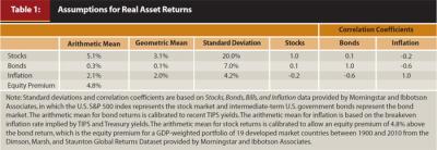
Bond yields are at historical lows, and some planners would like to use more typical average yields for long-term planning forecasts. While this may make sense for clients in the accumulation phase, it makes less sense in the post-retirement period. Current bond yields are the best predictors of subsequent bond returns. Even if bond yields increase in the subsequent years, this will imply capital losses for any client portfolio holding of medium or long-term bonds. Retirees must deal with sequence of returns risk, as any portfolio losses or spending of capital in early retirement has a disproportionate overall impact on the final retirement outcomes. In other words, even if real interest rates increase in five to 10 years, it is harder for today’s retirees to derive benefit than it is for today’s savers. As well, to provide a comparable basis for annuity prices, which are based on current bond yields, it is important to have matching assumptions for systematic withdrawals. This explains why current bond yields serve as a basis for the underlying assumptions in this research.
Retirement Financial Goals. As argued, retirees should not be narrowly focused on a singular goal to avoid financial wealth depletion. Financial goals for retirement can essentially be reduced to two competing objectives:
- Support minimum spending needs and lifestyle-spending goals as best as possible, however high they may be.
- Maintain a reserve of financial assets to support risk-management objectives such as protection from expensive health shocks, divorce, unexpected needs of other family members, severe economic downturns, etc., or to meet legacy objectives.
To the extent that greater spending requires more financial resources, and that more aggressive investment strategies imply greater upside wealth as well as greater downside spending risks, these objectives generally must be balanced in a manner that best supports client preferences.
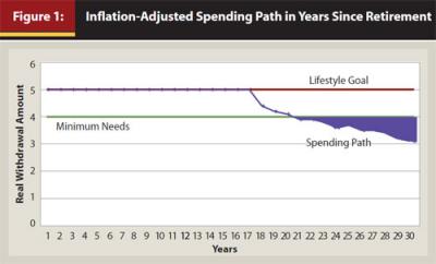
Utility measures translate spending into values that incorporate the concept of diminishing marginal enjoyment from spending increases. But defining an appropriate utility function for clients may be a difficult task. As an alternative here to operationalize how well a strategy meets spending goals, I propose summing the amounts of spending shortfalls created by a strategy. With Monte Carlo simulations for financial market returns, each strategy will have a distribution of spending shortfalls. Figure 1 shows how the shortfall calculation can be made for a single hypothetical spending pattern in one simulation. The focus is on when the spending level is forced below minimum needs. This shortfall area can be summed and then divided by the total lifetime minimum needs. With this information, we can calculate, in turn, the percentage of lifetime minimum needs that are met by the strategy. This measure provides the magnitude of shortfalls relative to a spending level the client views as essential. For clients, the minimum needs line could be less than the lifestyle goal, as shown in Figure 1, or it could be at the same level.
Academics thinking in terms of lifecycle finance theory will aim to make a clear distinction between minimum needs and lifestyle goals. Clients may be unhappy if an event such as a bad sequence of market returns makes their lifestyle goals unsustainable. But what could be truly disastrous is if their spending is forced to fall below a minimum level to meet basic needs.
Planners with practical client experience, though, may be more inclined to focus on spending below the lifestyle goal, as spending less than this may be viewed by the client as a failure regardless of any hypothetical minimum needs. For examples of the planner’s perspective, see Evensky, Horan, and Robinson (2011), Guyton (2011), and Kitces (2012). For the case study in the results, the minimum needs and lifestyle goals will be set equal out of respect for the planner’s perspective.
Efficient Frontier. The efficient frontier for retirement income described here identifies the specific allocations among various combinations of asset classes and financial products that maximize the reserve of financial assets for a given percentage of spending goals reached, or that maximizes the percentage of spending goals reached for a given reserve of financial assets. Though scalable, each client requires a personalized efficient frontier matching household characteristics including age, gender, marital status, health, life expectancy, desired spending patterns, and constraints about asset and product allocation (such as a restriction that no more than 50 percent of assets will be annuitized).
Customized expectations about the returns, volatilities, and correlations for asset classes and inflation, as well as mortality, can also be included, as can details about the current pricing of available retirement income tools. Different clients will desire different withdrawal rates for meeting basic expenses and for lifestyle-spending goals, and they will also have varying amounts of financial assets and varying inflation-adjusted income and fixed income from sources outside of the financial portfolio. After an efficient frontier of product allocations is constructed for these characteristics, clients can select one of the points on the frontier reflecting their personal preferences about the tradeoff between meeting spending goals and maintaining sufficient financial reserves. Results will be presented for a 65-year-old heterosexual couple (this distinction is relevant as gender affects survival probabilities) who are retiring and have already claimed Social Security (incorporating optimal claiming decisions into the framework will be left for subsequent research).
At retirement, assets are divided between stocks, bonds, inflation-adjusted SPIAs, fixed SPIAs, and VA/GLWBs. Each of these five components is simulated in 10 percentage point increments from zero to 100 percent, with 1,001 possible product allocations. For example, a product allocation of 20, 30, 10, 30, 10 means that at the retirement date, 20 percent of assets are invested in stocks, 30 percent in bonds, 10 percent into a real SPIA, 30 percent into a fixed SPIA, and 10 percent into a VA/GLWB. In this case, half of the assets remain in the financial portfolio with a fixed-asset allocation of 40 percent stocks and 60 percent bonds, as these represent the relative shares of the total assets devoted to stocks and bonds. For the portfolio of financial assets, annual rebalancing restores the fixed asset allocation.
To obtain each year’s spending amount (which is withdrawn at the start of each year), the maximum allowable amount is taken first from the annuitized financial products. If this sum exceeds what is needed to meet the lifestyle spending goal, then the excess funds are added to the financial portfolio. If the guaranteed income sources do not provide enough income to meet the lifestyle goal, then the remainder needed is withdrawn from the financial portfolio (stocks and bonds). Whenever fewer assets remain in the financial portfolio (stocks and bonds) than are needed to meet the spending goal, the client is unable to meet his or her full lifestyle-spending goal for that year. If that occurs, the client can only spend the income available from any annuities and Social Security. The contract value of the VA/GLWB rider is included as part of the financial assets plotted on the y-axis, but clients do not withdraw more than the allowable amount each year so as to avoid breaking the contract terms for the guarantee.
A single-premium immediate annuity allocation of 100 percent can still support a reserve of financial assets if the income received from the SPIA exceeds the lifestyle spending goal, as the excess is reinvested. In the case where the initial allocations to stocks and bonds are both zero, income returned to the investment portfolio in this manner is allocated to 100 percent stocks. Lifestyle goals and minimum needs are defined in real terms, while fixed SPIAs and VA/GLWBs only provide nominal guarantees (GLWB step-ups cannot generally be expected to keep pace with inflation). As inflation erodes the real value of the nominal income, the percentage of lifestyle goals these sources support declines.
Survival Probabilities. The outcome measures—remaining financial assets and percentage of lifetime spending needs which are satisfied—are calculated using survival probabilities from the Social Security Administration 2007 Period Life Table. The remaining financial-assets measure is the sum of remaining financial assets in each year of retirement, times the probability that the second member of the couple dies in that year. With this measure, the real value of remaining financial assets at death cannot be zero, as some retirees will die shortly after retirement when assets will surely remain. This measure is an ex ante estimate of remaining financial assets based on survival probabilities for an unknown lifetime. Meanwhile, the percentage of lifetime-spending needs that are satisfied is calculated as the sum of spending in each year as a percentage of the minimum spending need, times the probability that at least one member of the couple survives to that age.
Distribution of Outcomes. In presenting outcomes, the part of the distribution of outcomes that should be highlighted is not clear. For financial assets, should we focus on the mean amount, the median amount, or the remaining amount in a bad luck outcome such as the 10th percentile for values ranked from lowest to highest across the simulations? Likewise, the Monte Carlo simulations will produce a distribution of percentages of minimum spending needs that are met. Should we focus on the mean or median percentage of met needs across the simulations, or instead identify the percentage of needs met in a bad luck case such as the 10th percentile? Different possibilities should be investigated, though the issue becomes less important if the optimal strategies are fairly consistent between these different ways of measuring remaining financial assets and percentages of spending needs that are satisfied.
Results
Results are provided for a 65-year-old couple. Their Social Security benefit is equal to 2 percent of their retirement assets. Their lifestyle-spending goal is 6 percent of retirement assets, which requires them to use a 4 percent withdrawal rate above Social Security to meet their goal. Minimum needs are also 6 percent. Social Security is relevant because increasing the Social Security benefit will help support a higher percentage of spending needs being met, as it provides a further guaranteed income floor even when financial assets are depleted. Though higher Social Security benefits will not change the product allocations found on the efficient frontier, it will shift the frontier to the right, which could increase client comfort with choosing more aggressive allocations with a greater probability to increase financial asset holdings.
The efficient frontier for this case is shown in Figure 2, with the median value of remaining financial assets at death shown on the y-axis, and the 10th percentile bad-luck outcome of spending needs that could be satisfied shown on the x-axis. The figure illustrates how 1,001 different product allocations perform in meeting the two objectives. Moving toward the upper right hand corner of the figure is advantageous for retirees. A purple curve is added to show all of the product allocations consisting only of financial assets (stock and bonds). These outcomes represent some of the worst possible, demonstrating a clear role for partial annuitization to improve retiree outcomes, even in today’s low interest-rate environment. In particular, the red curve highlights most of the points on the efficient frontier. It shows the allocations between stocks and fixed single-premium immediate annuities.
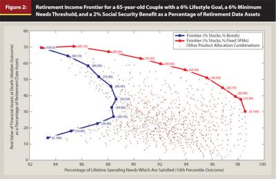
The results will vary when changing the personal characteristics and spending goals of the client. For instance, if spending needs require a withdrawal rate of only 1 percent of assets, then it is likely that spending needs will be met with any product allocation and the client can focus on the allocation that maximizes the median value of remaining financial assets: 100 percent stocks.
But in the particular case of Figure 2, the evidence suggests that optimal product allocations consist of stocks and fixed SPIAs, and clients need not bother with bonds, inflation-adjusted SPIAs, or VA/GLWBs. Though SPIAs do not offer liquidity, they provide mortality credits and generate bond-like income without any maturity date, and they support a higher stock allocation for remaining financial assets. Altogether, this allows a client to better meet both retirement financial objectives. Any of the product allocations on the efficient frontier represents a potentially optimal point, and clients can choose which one they think best balances their own objectives. Of course, any product allocations the client is not comfortable using could be removed and a constrained efficient frontier could be determined instead. For instance, clients may fear high stock allocations—especially if they may be tempted to sell after a market drop—or too much annuitization.
An interesting result is that fixed SPIAs dominate inflation-adjusted SPIAs in the retirement portfolio for this example. In personal correspondence, Joseph Tomlinson explains why this may be. Essentially, either because of a lack of competition or because of the difficulties of hedging inflation risks, inflation-adjusted SPIAs are not priced competitively with fixed SPIAs. Fixed SPIAs supply more inflation-adjusted income than real SPIAs until cumulative inflation sufficiently reduces the real value of the fixed SPIA income stream. With payout rates of 5.84 percent, the fixed SPIA payout is 51 percent larger than the 3.875 percent payout of the inflation-adjusted version. With inflation fluctuating around 2.1 percent, it takes almost 20 years, on average, for the income from the inflation-adjusted SPIA to grow larger.
Because using retirement-date assets to buy a fixed SPIA provides more income than needed until inflation sufficiently reduces the real value of the SPIA payments, and because excesses are invested in a portfolio of 100 percent stocks, a 100 percent allocation to a fixed SPIA can support more of the spending needs and result in the same median amount of financial reserves as a portfolio of 40 percent stocks and 60 percent bonds. Nevertheless, it is important to emphasize that clients with particular concerns about inflation may expect that the breakeven inflation rate is too low and may seek the additional protection provided by an inflation-adjusted SPIA.
Conclusion
Further refinements to this framework are needed to include a broader range of retirement-income strategies. These include optimization for the Social Security claiming decision, bond ladders and time segmentation approaches, delayed or laddered annuity purchases, deferred income annuities (longevity insurance), immediate variable annuities, long-term care insurance, life insurance, reverse mortgages, home equity loans, structured products based on derivatives to protect on the downside while maintaining some upside, and various other products. Equally important, taxes must be added to the analysis so that the efficient frontier can be calculated in after-tax terms. More detailed scenarios with varying asset-class assumptions, personalized client circumstances, and changing patterns for spending needs also can help to determine which sorts of findings are generalizable across a wide variety of circumstances. The approach described here provides the initial stages of a framework that can better inform planners and clients, and guide them in the direction of optimal retirement income strategies.
Acknowledgements: Many individuals provided me with useful feedback and discussions about the topics in this article. In particular, I wish to thank William Bernstein, Jason Branning, Tom Cochrane, Dirk Cotton, Michael Finke, Francois Gadenne, David Jacobs, Michael Kitces, David Littell, Manish Malhotra, Aaron Minney, Mike Piper, Dick Purcell, Bob Seawright, Joseph Tomlinson, and Michael Zwecher. I am grateful for financial support from the Japan Society for the Promotion of Science Grants-in-Aid for Young Scientists (B) #23730272.
References
Ameriks, John, Robert Veres, and Mark J. Warshawsky. 2001. “Making Retirement Income Last a Lifetime.” Journal of Financial Planning 14, 12 (December) 60–76.
Bengen, William P. 1994. “Determining Withdrawal Rates Using Historical Data.” Journal of Financial Planning 7, 4 (October): 171–180.
Chen, Peng, and Moshe A. Milevsky. 2003. “Merging Asset Allocation and Longevity Insurance: An Optimal Perspective on Payout Annuities.” Journal of Financial Planning 16, 6 (June): 52–63.
Cooley, Philip L., Carl M. Hubbard, and Daniel T. Walz. 1998. “Retirement Savings: Choosing a Withdrawal Rate That Is Sustainable.” American Association of Individual Investors Journal 20, 2 (February): 16–21.
Evensky, Harold, Stephen M. Horan, and Thomas R. Robinson. 2011. The New Wealth Management: The Financial Advisor’s Guide to Managing and Investing Client Assets. Hoboken, New Jersey: John Wiley and Sons.
Finke, Michael, Wade D. Pfau, and Duncan Williams. 2012. “Spending Flexibility and Safe Withdrawal Rates.” Journal of Financial Planning 25, 3 (March): 44–51.
Guyton, Jonathan T. 2011. “Study Suggests Link Between Planner Retirement Advice and Client Lifestyle Changes.” Journal of Financial Planning 24, 12 (December) 28–32.
Huang, Dylan W., Matthew M. Grove, and Todd E. Taylor. 2012. “The Efficient Income Frontier: A Product Allocation Framework for Retirement.” Retirement Management Journal 2, 1 (Spring): 9–22.
Kitces, Michael E. 2012. “The Problem with Essential Vs. Discretionary Retirement Strategies.” Nerd’s Eye View blog (May 30). www.kitces.com/blog/archives/329-The-Problem-With-Essential-Vs-Discretionary-Retirement-Strategies.html
Malhotra, Manish. 2012. “A Framework for Finding an Appropriate Retirement Income Strategy.” Journal of Financial Planning 25, 8 (August) 50–60.
Milevsky, Moshe A. 2009. Are You a Stock or a Bond? Create Your Own Pension Plan for a Secure Financial Future. Upper Saddle River, New Jersey: FT Press.
Milevsky, Moshe A., and Huaxiong Huang. 2011. “Spending Retirement on Planet Vulcan: The Impact of Longevity Risk Aversion on Optimal Withdrawal Rates.” Financial Analysts Journal 67, 2 (March/April): 45–58.
Pfau, Wade D. 2012. “Choosing a Retirement Income Strategy: A New Evaluation Framework.” Retirement Management Journal 2, 2 (Fall): 33–44.
Terry, Rory L. 2003. “The Relation Between Portfolio Composition and Sustainable Withdrawal Rates.” Journal of Financial Planning 16, 5 (May): 64–71.
Tomlinson, Joseph A. 2012. “A Utility-Based Approach to Evaluating Investment Strategies.” Journal of Financial Planning 25, 2 (February): 53–60.
Tresidder, Todd R. 2012. “Are Safe Withdrawal Rates Really Safe?” Journal of Personal Finance 11, 1: 113–142.
Vernon, Steve. 2012. “Retirement Income Scorecard: Immediate Annuities.” CBS News. (April 4). www.cbsnews.com/8301-505146_162-57408049/retirement-income-scorecard-immediate-annuities/