A Utility-Based Approach to Evaluating Investment Strategies

Journal of Financial Planning: February 2012

 

Joseph A. Tomlinson, FSA, CFP^® (joetmail@aol.com), is principal of Tomlinson Financial Planning LLC in Greenville, Maine. He is both an actuary and a financial planner, with recent articles published in Financial Planning Magazine, Retirement Income Journal, and Advisor Perspectives. He is a member of the Society of Actuaries Committee on Post-Retirement Needs and Risks, and recently headed a major project on managing retirement decisions.

Executive Summary

• Previous studies on asset allocation for retirement have typically focused on the probability of running out of money as the key evaluation measure. In this article I develop an approach that broadens the measures to also include the magnitude of plan failure and expected bequest amounts.
• I combine these three financial measures into a proposed single utility measure. To provide a utility measure for plan failures, I use the behavioral concept of loss aversion. In this context, loss aversion recognizes that running out of money weighs much more heavily than being able to leave a bequest. Results of an informal survey are used to gauge loss aversion.
• My primary objective in writing this article is not to make specific asset allocation recommendations, but to help lay the groundwork for development of a new utility-based approach to making such recommendations.
• The analysis uses a specific retirement example to demonstrate how the utility concepts are developed and applied. The available asset classes are stocks, bonds, and an inflation-adjusted immediate annuity.
• The results demonstrate the importance of individual loss aversion characteristics in setting an asset allocation strategy. Also, the assumption about future stock returns is critical. Optimal allocations tend toward 100 percent stocks or 100 percent annuities depending on loss aversion and the stock return assumption. Allocations that mix stock and bond investments tend to perform worse on the utility measures.
• The article concludes with suggestions for future steps in development.

Over the past two decades, this Journal has featured numerous articles on managing investments in retirement portfolios. These articles have mostly focused on safe withdrawal rates and used the probability of running out of money (plan failure) as the primary measure of retirement plan performance. These articles have also examined asset allocation for retirement portfolios, but that has not been their main focus.

In this article, I turn the attention to asset allocation and bring in two additional measures of retirement plan performance: the magnitude of plan failure and expected bequest amounts. The main part of this work involves the development of a utility measure that combines all three financial measures. I show how this proposed utility measure can be used to evaluate a range of investment strategies. Particular aspects of my approach include:

• Using stochastic mortality rather than managing to a fixed time horizon
• Including an inflation-adjusted immediate annuity as a third asset class in addition to traditional stock and bond investments
• Incorporating specific recognition of loss aversion to measure the utility of varying magnitudes of plan failure
• Incorporating results from an informal survey on loss aversion

This study is deliberately limited in scope. I use a single example and carry it through the analysis. At this stage, the development of a new way of measuring retirement plan performance is more important than the numbers generated or the preliminary conclusions about different investment strategies. My aim is to provide a fresh view on important issues, and my hope is that this work will spur others to refine and extend the research.

Gains and Losses

Before getting into the actual analysis, it is worth discussing the particular gain and loss concepts I will use. If we think of retirement outcomes and focus on the end of life, I use gain to mean that an individual does not deplete funds and has money left over for a bequest. The amount of gain is the amount of the bequest. I use loss to refer to a plan failure where the individual runs out of money prior to death. Such a loss is calculated as a negative bequest, and its size provides a measure of the magnitude of the plan failure. For example, running out of money at age 75, but living to age 95, would result in a sizable loss or negative bequest.

The development of utility measures involves translating the financial outcomes into measures of satisfaction. The concept of loss aversion is applied in developing the utility measures to recognize that losses (negative bequests) have a much bigger impact on well-being than gains (positive bequests) of similar amount.

It is worth noting that the concept of loss aversion as I use it is somewhat different than in other economics work. When Kahneman and Tversky did their Nobel Prize-winning work on prospect theory and loss aversion, they demonstrated how a narrow framing of choices could lead to a heightened aversion to losses and irrational decision making. For this analysis, I use a broad frame that considers the whole retirement period. In this context, it is rational to recognize the very different impacts of positive versus negative retirement outcomes.

Retirement Planning Example

The analysis in this paper is based on an individual at the beginning of retirement, with the following assumptions:

• Longevity: Variable life spans with a 20-year life expectancy
• Expenses: Basic living expenses, level from year to year in real terms (increasing with inflation)
• Annuity Option: Inflation-indexed immediate annuity with an initial payout rate of 5.05 percent per year (payable monthly)
• Investment Returns: Stocks, 6.5 percent real return, 20 percent annual standard deviation; risk-free bonds, 1 percent real return, 0 percent standard deviation

The longevity assumptions would be appropriate for a 65-year-old male in good health based on the Society of Actuaries (SOA) RP-2000 mortality tables and SOA recommended improvement scales (calculations done by the author). The annuity rate is for a 65-year-old male from Income Solutions via the www.vanguard.com website (rates as of 9/25/11). Stock return estimates were based on the Fernandez et al. (2011) worldwide survey of risk premium estimates, with input from 6,000+ economists and other investment professionals. The standard deviation estimate came from history for the S&P 500 from 1926–2010. The risk-free bond rate was based on historical averages for Treasury Inflation Protected Securities (TIPS) graded down to recognize recent lower rates.

The estimate of future stock returns turns out to be the most critical variable affecting this study’s conclusions. The 6.5 percent real return (derived by adding the Fernandez et al. (2011) 5.5 percent risk premium estimate to the 1 percent risk-free bond rate) is about 2 percent lower than the average real return for U.S. stocks over the period 1926–2010. Despite this conservatism, there are compelling arguments that future returns may be even lower. Later in the study, I show results for an alternative scenario with real stock returns of 4.5 percent.

The individual in this example is assumed to have just enough assets to purchase an annuity with payouts that match the portion of daily living expenses not already covered by annuity-like payments (such as Social Security benefits). The analysis of the various asset allocations uses a 5.05 percent inflation-adjusted withdrawal rate, which matches the annuity. Monte Carlo simulations are used to project outcomes.

Financial Results

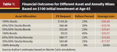
Table 1 shows estimated financial outcomes based on different stock/bond mixes and stock/annuity mixes. The “PV Bequest” column shows the present value of expected remaining funds at time of death per $100 of initial investment—after taking lifetime systematic withdrawals or annuity payments. Present values are calculated using the 1 percent risk-free rate, and amounts are in current dollars. “Failure Percent” is the probability that the strategy runs out of money before the time of death. “Average Loss” is the average negative PV bequest (to measure the magnitude of loss) for the subset of cases that fail.

These results were calculated using a VBA program developed by the author to do Monte Carlo projections. The program runs 1,000 40-year investment scenarios for each asset allocation. Each run starts with $100 at age 65, with monthly increases (or decreases) based on randomly generated real investment returns and monthly withdrawals equal to $5.05/12. Projected bequest values (positive or negative) are calculated at the end of each month. Mortality variability is brought in by weighting the outcomes by the probability of death in each month. The results shown in Table 1 are averages for the 1,000 investment scenarios generated for each asset allocation.

A few comments about Table 1:

• The inflation-indexed annuity shows no PV bequest or failures. The annuity provides inflation-indexed payments that cover expenses, and the payments last for life.
• The 100 percent stock allocation produces the highest PV bequest because that allocation has the highest expected return.
• Failure percentages reflect both longevity risk and investment volatility. In particular, note the high failure rate (45 percent) for the 100 percent bond allocation. Even though the investments are risk free, those who live longer than average generate losses.
• Failure percentages for all strategies except 100 percent annuity are above 20 percent, reflecting the somewhat aggressive withdrawal rate (5.05 percent) compared with more typical planning guidelines such as the “4 percent rule.”
• The stock/annuity mixes can be thought of as smaller versions of the 100 percent stock case—basically the outcomes for 100 percent stock multiplied by the stock percentage (65 percent or 35 percent). The failure percentages remain the same as 100 percent stock because the mix strategies will still fail as often but produce smaller dollar losses.

The first comment about the annuity merits some additional discussion. Immediate annuities are often viewed as producing losses for those who die early and gains for those who live a long time, whereas I am portraying no gain or loss regardless of the length of life. This is an issue of framing or context. My view of gains and losses considers both retirement income and retirement expenses. If one thinks of an annuity as providing income to meet basic living expenses, both the income and the expenses will end at death. There is no bequest, but there is also no chance of plan failure. Mine is a broader framing than the view that focuses only on the annuity investment. There is no “right” or “wrong” framing, but I believe that including both the income and the expenses is more appropriate for evaluating asset allocation strategies for retirement.

An exhibit like Table 1 could be used to make recommendations about asset allocation and whether to purchase annuities. The problem is that three different variables need to be brought into the decision. This naturally leads to the question of whether a more informative decision tool could be developed by combining the measures. To do this we need to shift our focus from pure financial outcomes to the fuzzier concept of the satisfaction associated with those outcomes. We need to develop a utility measure.

Building a Utility Function

My objective is to build a utility function to translate the Table 1 financial outcomes into utility measures. Figure 1 shows the general shape of the utility function I am proposing.

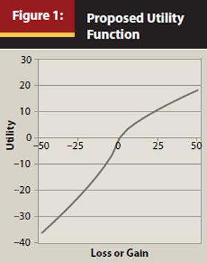
The general shape of the utility function is more important than the actual numbers. Utility functions are designed to show a ranking of preferences rather than unique quantities. Here are a few key points about the shape, some of which will merit further discussion:

• The curve has a positive slope throughout—gains are preferred over losses; more is better for gains and less is better for losses
• The curve passes through the origin—an arbitrary choice so that losses are given a negative utility score and gains a positive score
• There is a kink at the origin suggesting that individuals weigh losses more heavily than gains
• In the gains region, the slope decreases as gains increase (a shape mathematicians call concave) reflecting diminishing marginal utility or risk aversion (individuals are assumed to prefer a $100 gain to an equal chance of zero or $200)
• In the loss region, the curvature is an amplified mirror image of the curvature in the gains region, which keeps the same weighting between gains and losses throughout

The third bullet is particularly important for this process of assigning utilities to financial outcomes. Kahneman and Tversky, in their pioneering work on behavioral economics, introduced the concept of loss aversion, hypothesizing that individuals place more weight on losses than can be explained by risk aversion—hence the kink at the origin. Tversky and Kahneman (1992) carried out experiments in which they examined participants’ subjective trade-offs between hypothetical small dollar gains and losses, and found about a 2 for 1 weight for losses versus gains.

The gain and loss situation for this analysis is different in character from the experiments carried out by Kahneman and Tversky. Here the stakes are higher, and the nature of losses is different from gains. A “loss” in this case means plan failure (running out of money during retirement), and a “gain” means being able to leave a bequest.

Loss aversion for this particular analysis can be thought of as a combination of Kahneman and Tversky’s loss aversion and the negative of bequest motivation. For example, someone who is average in their aversion to suffering financial losses, but has no motivation to leave a bequest, will score higher than average on the loss aversion measure I am using. Given the difference in impact on personal well-being of gains versus losses in this analysis, it would seem reasonable that loss aversion should exceed 2 for 1. But the question is, “By how much?”

An Informal Survey

To get a rough idea of how individuals might assess this trade-off, I developed a brief survey and used it with 36 participants. Those surveyed were told to assume that they were retiring at age 65 and had earned a pension from work of $25,000 per year with inflation adjustments. The pension plus Social Security of $15,000 per year would be just sufficient to live comfortably, but not extravagantly, in retirement. They were next told that, instead of the pension, their employer was willing to offer a cash settlement at retirement they could invest and use for systematic withdrawals in the same amount as the pension—$25,000 per year, increasing with inflation. The risks in taking the cash settlement were described in the following simplified way.

• A 50 percent chance of plan failure leaving nothing but Social Security for the last two years of life—not a starvation scenario, but a huge disruption in life circumstances
• A 50 percent chance that investments do well, providing sufficient funds to match the pension payouts and generating additional funds for a bequest

The question they were asked was, “How large would the bequest need to be to make it worth taking the cash settlement?” In other words, how large would the bequest (gain) need to be to make up for a potential $50,000 loss?

Of the 36 responses, 12 were for $250,000 (5:1) and 11 were for $500,000 (10:1), so they were tightly clustered. The seven responses above $500,000 ranged from $760,877 (from a fellow actuary!) up to $2 million, and there were two answers that “no amount is enough.” Of the six respondents below $250,000, there were three individuals willing to accept an even trade at $50,000, one at 2:1 ($100,000), and two at $200,000.

Twelve of the 36 respondents were shown the results of the survey, and then asked a follow-up question. They were told that the same circumstances applied as for the first question, except to assume that they were wealthier and would leave a certain $500,000 bequest if they took the pension. The alternative was to take the cash settlement where outcomes were described as a 50 percent chance of leaving a bequest of $450,000 (a $50,000 loss) and a 50 percent chance of leaving a bequest of (X plus $500,000). The question was, “How large would X need to be to make it worth taking the cash settlement?”

Under this scenario, losses would only affect bequest amounts and have no impact on life circumstances. Not surprisingly, the chosen Xs clustered around a smaller number than before. One-hundred thousand dollars was chosen by 8 of the 12, with three higher (up to $250,000) and one at $50,000. This result is roughly consistent with Kahneman and Tversky’s findings of an approximate 2:1 loss aversion ratio.

Shape of the Utility Function

This survey provided data points for loss aversion ratios to use in building the utility function. I also needed to come up with shapes for the utility curves for gains as well as losses. For gains, it seems reasonable that the utility function should be an increasing function with decreasing slope (concave). Various mathematical functions can be used to portray this shape. Kahneman and Tversky used a simple power function of (Gain ^ alpha, in Excel terminology), where alpha is a constant between zero and one.

For losses, Kahneman and Tversky suggested “risk seeking” rather than “risk aversion,” so that the curve becomes the convex mirror image of the curve for gains. They refer to shape of the overall utility function as exhibiting diminishing sensitivity as one moves away from the zero reference point. For example, the difference in utility from no plan failure at all and one year without income would be greater than the difference between 9 years without income and 10 years without income.

To come up with an estimate of the alpha exponent for gains and losses, Kahneman and Tversky used a computer questionnaire on a group of 25 graduate students. They asked questions such as, “How much would you accept as a sure outcome in place of a gamble with a 50 percent chance of receiving $50 and a 50 percent chance of receiving $100?” They also asked similar questions about losses. Based on the responses, they came up with an estimated alpha of .88 and found that this number gave a good fit for both gains and losses.

Their experiments included both long-odds cases—such as lotteries—and cases in which the odds were more even. They noted that the even-odds cases fit better with a lower alpha. I believe such cases are more representative of retirement decisions, so I examined the subset of their cases in the 25/75, 50/50, and 75/25 range and developed an estimated alpha of .74. This provided a good fit for both gains and losses, and I used this alpha value to estimate utilities. (A natural extension of this research will be to do experiments with live subjects where the questions relate explicitly to retirement trade-offs.)

We now have all the assumptions needed to fully define utility curves and translate financial outcomes into utility measures.

Utility Results

Table 2 shows the results for the same asset allocations and stock/annuity mixes shown in Table 1. The 100 percent annuity strategy serves as the base case, and various asset allocation strategies are measured against it. Positive numbers indicate that a systematic withdrawal strategy using the specified asset allocation or stock/annuity mix produces more expected utility than the 100 percent annuity strategy, and negative numbers favor the annuity strategy.

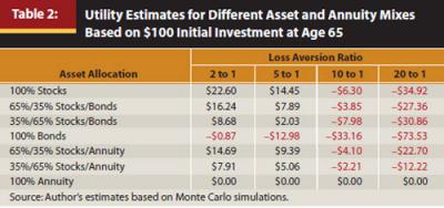
The results were produced from one additional step in the Monte Carlo projections used to generate Table 1—dollar bequest values were translated into utility units. For positive outcomes, the translation was (Bequest ^ .74, in Excel terminology). For negative outcomes, this calculated value was multiplied by the loss aversion ratio.

Before discussing the numbers, it is worth shedding light on the relationship between Table 2 and Table 1. Using the 100 percent stock allocation as an example, the expected PV bequest in Table 1 was $124.26. With a loss aversion of 2:1, the expected utility for 100 percent stocks is $22.60, which can be thought of like a PV bequest measure in a new “utility currency” in which losses have twice the weight of gains. As we move to the right on Table 2, the numbers get smaller (or go negative) as successively higher weights are applied to losses.

The results shown in Table 2 pass a commonsense test—negative numbers on the far right suggest an annuity strategy for individuals with a strong aversion to financial losses (and/or lacking bequest motivation), and positive numbers on the left suggest systematic withdrawals with a high stock allocation for less loss-averse individuals. Because 5:1 and 10:1 represent the average loss aversion from the survey, I have used 20:1 to represent a particularly loss-averse individual and 2:1 for an individual who has enough wealth to eliminate any concerns about running out of funds.

Table 2 Findings

It would be presumptuous to state general conclusions based on a single example and a single withdrawal rate, but even this limited test provides some findings worth thinking about.

Loss aversion affects the choice of strategy. It is clear that the choice of buying an annuity versus taking withdrawals from savings is a function of loss aversion (and/or lack of bequest motivation).

No clear winner is evident for annuities versus withdrawals from savings. The split where the utility numbers go from positive to negative falls at the mid-range of loss aversion, given that 5:1 and 10:1 were the most popular picks. It is perhaps surprising that the annuity strategy does not do even better, because the design of this example is somewhat biased toward annuities. The client is financially constrained, requiring an aggressive withdrawal rate with a significant risk of plan failure. Another pro-annuity bias is that the expenses are assumed completely predictable and perfectly matched with an inflation-adjusted annuity payout. Nonetheless, these findings do favor taking withdrawals from savings for the less loss-averse individuals.

Utility maximizing strategies are either 100 percent stocks or 100 percent annuities depending on loss aversion. For those loss aversion levels that do not favor annuities, the 100 percent stock allocation beats the various mixes of stocks with bonds or annuities. It should not be a surprise that 100 percent stock produces the best expected financial outcomes (see Table 1), but it may seem curious that it also produces the best utility outcomes. Other studies on safe withdrawal strategies such as Bengen (1994), Guyton (2004), and Kitces (2008) have all recommended greater than 50 percent stock allocations, but none have pushed all the way to 100 percent. However, those studies focused only on probabilities of running out of money, whereas my utility measure also considers bequest values. Bringing in this added factor tilts the outcome in favor of stocks.

For the higher loss aversion levels that favor annuities, it is worth noting the 65 percent/35 percent stocks/bonds does better than 100 percent stocks, although neither does as well as 100 percent annuity. So for these cases we see how more conservative allocations might be preferred to 100 percent stocks if annuities were not an available option. The message seems to be that if one seeks safety with fixed-income investments, the annuity with its longevity guarantees works better than bonds.

The all-bond strategy looks like a big loser. A high proportion of retirees own no stocks whatsoever, as shown by Coile and Milligan (2006), even before the financial crisis. Investing in bonds may look like a safe strategy when a fixed life expectancy is assumed. However, the picture changes completely when variable mortality is introduced. Table 1 shows a 45 percent failure rate for such a strategy, and the Table 2 utility measurements show that the 100 percent bond strategy performs significantly worse than any other strategy. Table 2 also demonstrates that a conservative allocation, such as 35 percent/65 percent stock/bond, produces mediocre expected outcomes.

The equity premium is uncertain. I used a consensus forecast for return advantage for stocks over bonds (the equity premium). However, there is certainly a case to be made that the future equity premium will be even lower than the forecast. PIMCO has been in the news for the past few years with its prediction that we have entered a “new normal” and face a long period with reduced rewards for risk-taking. Market valuations may also be a concern. The PE/10 measure, popularized by Robert Shiller, is currently around 20, based on the S&P 500 at 1,200, compared with a long-term average of 16.4. A recent article in the Economist¹ cites three different forecasts of future real returns for the American stock market ranging from 0.6 percent to 4.5 percent. It turns out that the choice of equity premium assumption is critical for this type of analysis.

Impact of a Lower Equity Premium

I find the arguments for lower returns compelling, and have therefore repeated the utility calculations with real stock returns lowered from 6.5 percent to 4.5 percent.

Systematic withdrawal loses most of its utility-maximizing advantage under the lower stock return assumption, except for the least loss-averse individuals. See Table 3.

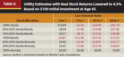
Perhaps the most important point from the comparison of Tables 2 and 3 is that the choice of equity premium assumption can tip the scales regarding whether to recommend annuities. This uncertainty creates a dilemma for planners, particularly when advising financially constrained clients.

It might be possible to sidestep this dilemma if there were a way to provide some downside protection for systematic withdrawal strategies. The good news is a product is already designed to do this—the guaranteed lifetime withdrawal benefit, a popular rider option for variable annuities. The bad news is this rider, as it is currently structured and priced, does not really do the job. However, this product structure could be very useful if it became available in a low-cost, index-funds version, with an inflation guarantee, but without the commission loads and the charges for active management.

Other Considerations

Behavioral considerations. Although 100 percent stocks produced higher utility values than stock/bond mixes for the less loss-averse cases, we would not expect advisers to be rushing to make such recommendations. The best long-term retirement strategy might prove unworkable given the all-too-human tendency to bail out in down markets. Given behavioral considerations, it may make sense to determine an optimal strategy and then dial back as necessary to an allocation that the client, with adviser coaching, can maintain through the market ups and downs.

Mean reversion of stocks. The stock returns I projected using Monte Carlo analysis assumed independence of year-by-year returns—that stock returns follow a random walk. There is considerable evidence that stock returns have historically shown mean reversion (Siegel 1998) and that long-term variability of returns has been significantly less than a random walk would have predicted. If such mean reversion continues into the future, that would improve outcomes for systematic withdrawal portfolios heavily concentrated in stocks compared with the outcomes I have projected.

Annuity concerns. There is a role to be played by immediate annuities, and how big that role is depends on client characteristics and economic assumptions. However, even for those clients whose main concern is outliving their funds, annuities are not likely to be an easy sell. Individuals are naturally averse to making large, irreversible financial commitments. Other concerns about annuities include:

• Lack of liquidity and flexibility
• Current low interest rates, which affect annuity payout rates
• Potential regret if an annuity is purchased and rates subsequently rise significantly
• Potential regret (for heirs) if the individual purchasing the annuity lives a shorter-than-expected life
• Publicity about heavy sales charges in annuities (although immediate annuities are an exception)
• Pricing margins built into annuities for adverse selection (healthy lives)
• High charges for the inflation-adjustment feature compared with market measures of inflation expectations
• Insurance company credit risk

Many of these concerns can be addressed, although doing so would require a separate article. Suffice it to say, determining the best strategy for a client and then selling that strategy can be challenging tasks.

Key Takeaways for Planners

This article provides a description of work in progress and does not yet offer specific prescriptions for planners. Perhaps the most important point that can be gleaned so far is that retirement planning needs to move beyond one-size-fits-all guidelines. Clients will naturally differ in loss aversion characteristics, and those differences will have a big impact on appropriate asset allocations.² We are moving in the direction of a much more individualized approach to retirement planning.³

Here are a few key areas for development to move toward providing tools and techniques planners can apply in practice:

• Formal survey research, focused specifically on retirement, will be needed to provide a better assessment of averages and ranges for the input variables needed to build utility functions.
• For individual client work, planners will need risk tolerance assessment tools that go beyond those provided today. The tools will need to be changed or expanded to gather the information needed to come up with individual loss aversion multipliers, risk aversion coefficients (curvature of utility function), and information about bequest motivation, including the trade-off of consumption versus bequests.
• Development work is needed to provide measures of the utility of consumption, so that comprehensive tools can be developed to address both asset allocation and withdrawal rates. Individual client characteristics will be an important input in actual planning.
• To be useful to planners, these research developments will need to be transformed into user-friendly planning software. Such software will need to handle a full array of retirement products, including regular investments, immediate annuities, variable annuities with living benefits, and deferred-income annuities.
• The changes in retirement planning that emerge will point up the need for new products and changes to existing products—particularly for products that carry investment and longevity guarantees.

The potential is building to create better tools for retirement planning. With 76 million baby boomers just beginning to retire, these developments are certainly timely.

Endnotes

1. The Economist staff. 2011. “I Wouldn’t Start from Here.” The Economist (October 15–21): 80–81.
2. It’s worth noting ongoing work by Wade Pfau, Ph.D., CFA, who has written for this Journal, demonstrating that optimal withdrawal strategies also need to take individual characteristics into account, and utility maximization can be applied there as well.
3. There is an enormous body of literature on the topics of utility theory, prospect theory, annuities, systematic withdrawal, asset allocation, and retirement income. A very useful summary of the relevant work for retirement planning is: Webb, Anthony. 2009. “Providing Income for a Lifetime: Bridging the Gap Between Academic Research and Practical Advice.” AARP Public Policy Institute.

References

Bengen, William P. 1994. “Determining Withdrawal Rates Using Historical Data.” Journal of Financial Planning 7, 4: 171–180.

Coile, Courtney, and Kevin Milligan. 2006. “How Household Portfolios Evolve After Retirement: The Effect of Aging and Health Shocks.” Working Paper No. 12391. Cambridge, MA: National Bureau of Economic Research.

Fernandez, Pablo, Javier Aguirreamalloa, and Luis Corres. 2011. “U.S. Market Risk Premium Used in 2011 by Professors, Analysts, and Companies: A Survey with 6,014 Answers.” Working Paper WP-918. Madrid, Spain: IESE Business School (University of Navarra).

Guyton, Jonathan T. 2004. “Decision Rules and Portfolio Management for Retirees: Is the ‘Safe’ Initial Withdrawal Rate Too Safe?” Journal of Financial Planning 17, 10 (October): 54–62.

Kitces, Michael. 2008. “Resolving the Paradox—Is the Safe Withdrawal Rate Sometimes Too Safe?” The Kitces Report (May): 1–13.

Siegel, Jeremy J. 1998. Stocks for the Long Run. 2nd ed. New York: McGraw Hill. 12.

Tversky, Amos, and Daniel Kahneman. 1992. “Advances in Prospect Theory: Cumulative Representation of Uncertainty.” Journal of Risk and Uncertainty 5, 4 (October): 297–323.

Acknowledgments: I would like to thank the Journal’s anonymous reviewers for their helpful suggestions. This article has also benefited from discussions with Wade Pfau, Ph.D., CFA, who does research on retirement planning issues and writes for this Journal.