Reversing the Conventional Wisdom: Using Home Equity to Supplement Retirement Income

Journal of Financial Planning: February 2012

 

Barry H. Sacks, J.D., Ph.D., is a practicing tax attorney in San Francisco, California. He has specialized in pension-related legal matters since 1973 and has published numerous articles in legal journals.

Stephen R. Sacks, Ph.D., is professor emeritus of economics at the University of Connecticut. He maintains an economics consulting practice in New York and has published articles on operations research.

Executive Summary

• This paper examines three strategies for using home equity, in the form of a reverse mortgage credit line, to increase the safe maximum initial rate of retirement income withdrawals.
• These strategies are: (1) the conventional, passive strategy of using the reverse mortgage as a last resort after exhausting the securities portfolio; and two active strategies: (2) a coordinated strategy under which the credit line is drawn upon according to an algorithm designed to maximize portfolio recovery after negative investment returns, and (3) drawing upon the reverse mortgage credit line first, until exhausted.
• A three-spreadsheet stochastic model is described, with one spreadsheet incorporating each strategy. The three spreadsheets are run simultaneously, with the same investment performance and withdrawal amounts in each. The cash flow survival probability over 30 years is determined for each strategy, and the comparisons are presented graphically for a range of initial withdrawal rates. We find substantial increases in the cash flow survival probability when the active strategies are used as compared with the results when the conventional strategy is used. For example, the 30-year cash flow survival probability for an initial withdrawal rate of 6 percent is only 55 percent when the conventional strategy is used, but is close to 90 percent when the coordinated strategy is used.
• The model also shows that the retiree’s residual net worth (portfolio plus home equity) after 30 years is about twice as likely to be greater when an active strategy is used than when the conventional strategy is used.

The overriding objective for many retirees is to maintain cash flow throughout their retirement years, to avoid “running out of money” in their later years. Cash flow survival is the central theme of this article.

Although more than half of retirees age 65 and older (64 percent) get at least half of their retirement income from Social Security,¹ there is a significant portion of the population of retirees whose primary source of retirement income is a portfolio of securities, often in a pre-tax account such as a 401(k) plan or a rollover individual retirement account (IRA). We will refer to any such account, whether pre-tax or after-tax, as an “account.”²

It has long been accepted that the maximum safe (or “safemax”) annual withdrawal from an account begins with a first year’s withdrawal equal to between 4.0 percent and 4.25 percent of the initial portfolio value. Subsequent years’ withdrawals then continue at the same dollar amount each year, adjusted only for inflation (thus maintaining constant purchasing power). In this context, the term “safe” means a 90 percent or greater probability that the account will have sufficient assets to make such annual payments for at least 30 years.³

Many retirees find that the safemax amount of annual withdrawal is uncomfortably limiting and therefore tend to draw more than that amount. This article considers three strategies for coping with the economic risk, the risk of exhausting cash flow, that derives from taking withdrawals in excess of the safemax amount.

The three strategies considered all involve the use of home equity as a supplement to withdrawals from the account. The conventional wisdom holds that home equity, drawn upon in the form of a reverse mortgage (discussed below) or similar product,⁴ should be used as a last resort, only if and when the account is exhausted.⁵ This is a rather passive approach. We show that the probability of cash flow survival is substantially enhanced by reversing the conventional wisdom. In particular, we show that cash flow drawn from home equity using either of two more “active strategies,” in conjunction with withdrawals from the account, yields cash flow survival probability substantially greater than the more passive approach of using home equity as the last resort (the “conventional strategy”).

One of the active strategies is quite simple: a straightforward reversal of the conventional wisdom. In this strategy, a reverse mortgage credit line is established at the outset of retirement, and the credit line is drawn upon every year to provide the retirement income until it is exhausted. Only after the reverse mortgage credit line is exhausted are withdrawals taken from the account. This is the “reverse-mortgage-first strategy.”

The other active strategy is more sophisticated. It also uses a reverse mortgage credit line, but withdrawals from the credit line are taken in some years and not others. The withdrawals are taken according to an algorithm described later in this paper. Because the algorithm consists of coordination between the account and the line of credit, this strategy is termed the “coordinated strategy.”

Some Fundamental Considerations

Before we examine the effect of these strategies, it is important to emphasize that a reverse mortgage is not necessarily a useful vehicle for every retiree who has substantial home equity. A retiree whose primary source of retirement income is a securities portfolio and who also has substantial home equity must decide early in retirement whether to live within the safemax limit set by his or her portfolio. This decision is a fundamental component of overall retirement planning.

The decision process includes, among other things, the balance between the desired consumption level, on the one hand, and the bequest motive and/or the economic safety net of the home equity, on the other hand. The decision process also must take into account the degree of economic discipline required to live within the safemax limit.

If the retiree does conclude that he or she would, on balance, prefer to live beyond the safemax level and wants to remain in his or her home as long as possible, a reverse mortgage, including its substantial costs, is one tool to consider. Although the costs do not affect the retiree’s cash flow, they become part of the debt, along with the cash drawn and interest accrued, to significantly reduce the equity remaining when the retiree ultimately leaves the home.

The thrust of this article is not whether a retiree should take a reverse mortgage. Rather, if the retiree has determined to live beyond the safemax level of the portfolio and consequently needs to rely on home equity for cash flow to supplement the cash from the portfolio, this paper shows how the active strategies provide substantially greater long-term cash flow survival probability than the passive conventional strategy.

The Rationales for the Two Active Strategies

In the cases in which withdrawals from a securities portfolio lead to exhaustion of the portfolio, it is most often because the investment performance in the early years of withdrawal has been weak or negative. Thus, the losses or even the weak gains in the early “down” years, coupled with the withdrawals in those years, lead to the portfolio’s not having enough assets to recover in the later “up” years. The two active strategies are designed to offset that situation by either: (1) allowing the portfolio to grow by taking no withdrawals from it during any of the early years of retirement until the reverse mortgage credit line is exhausted (the reverse-mortgage-first strategy); or (2) allowing the portfolio to grow during the early years of retirement by taking no withdrawals from it only in those early years that follow years in which the portfolio’s performance was negative (the coordinated strategy).

Rationale for the Reverse-Mortgage-First Strategy. The reverse-mortgage-first strategy allows the account to grow during the early years of retirement. Generally, over the years that the reverse mortgage credit line is drawn upon and exhausted, the portfolio will grow at an average rate greater than inflation. Therefore, in the year following the one in which the reverse mortgage credit line is exhausted, the withdrawal will be a smaller percentage of the portfolio than the initial withdrawal would have been at the outset of retirement. Furthermore, by that time, the retiree’s life expectancy is less than it was at the outset of retirement. These two factors together favor the lifetime cash flow survival of the portfolio.

Rationale for the Coordinated Strategy. The coordinated strategy is based on the following algorithm: at the end of each year, the investment performance of the account during that year is determined; if the performance was positive, the next year’s income withdrawal is from the account, and if the performance was negative, the next year’s income withdrawal is from the reverse mortgage credit line.⁶ In this way, the account is spared any drain (resulting from withdrawal) when it is “down” because of its investment performance. This leaves the account more assets to “recover” in subsequent “up” years. This is done when most necessary—in the early years of retirement, so the account grows before the reverse mortgage credit line is exhausted.⁷

It is not obvious whether the cash flow would survive just as long, or longer, under the reverse-mortgage-last strategy as under either of the active strategies. The only way to compare the results of the three strategies is with a quantitative test.

The Analytic Technique

To compare the two active strategies with the reverse-mortgage-last strategy, we have constructed a spreadsheet model. The model has the following input parameters:

1. The initial value of the retiree’s account
2. The value of the retiree’s home (we assume that the home is not encumbered by any mortgage debt)
3. The initial withdrawal rate as a percentage of the account value

The model uses three worksheets run simultaneously. The three worksheets are identical in all respects (including the investment performance of the account, the rate of inflation, and the amount drawn by the retiree) except for the strategy used to determine whether retirement income is withdrawn from the account and/or the reverse mortgage credit line.

On each worksheet, the calculations of investment gain or loss, and of retirement income withdrawal, are performed for each year in a 30-year period. The investment gain or loss is determined stochastically, as is the inflation adjustment to the withdrawal amount.⁸ In the course of the calculations, the cash flow either survives or it does not survive. It survives if there is enough money from the account and/or the reverse mortgage credit line to make the required income withdrawals for all 30 years.

The 30-year calculation is repeated 1,000 times. In a certain number of those repetitions, the cash flow will survive for 30 years, and in the other repetitions it will not. (As noted above, the two most significant determinants of cash flow survival are the initial withdrawal rate and whether the higher investment earning years occur early or late in the 30-year sequence.) In each of the 1,000 repetitions, the initial withdrawal rate is the same, and the average investment return is the same, but the sequence of investment returns, being randomly selected, is not the same in each repetition of the calculation. A simple count is made of cash flow survival over the 1,000 trials (with the three worksheets run simultaneously in each trial and results of the 1,000 trials shown on a histogram for each worksheet). The percentage of the repetitions in which the cash flow survives is termed the “cash flow survival probability.”⁹

Our primary focus is on the comparison of the cash flow survival probabilities of the three strategies. A secondary focus is on the comparison among the three strategies of the retiree’s residual net worth at the end of 30 years.

The Portfolio

The securities portfolio held by the account, in all the analyses and results shown, is a 60/40 portfolio comprised of the following indices, in the following proportions:

• Equities (60 percent): S&P 500, 40 percent; CRSP 6–10, 10 percent; and MSCI EAFE, 10 percent
• Fixed Income (40 percent): Bar Cap Int.-Term Gov’t./Credit Bond Index, 15 percent; U.S. 1 Year Const. Maturity, 15 percent; Bar Cap Long-Term Gov’t./Credit Bond Index, 10 percent

In our Monte Carlo simulations, we used investment return data on these indices from the 37-year period from 1973 through 2009. This captured several periods of significant volatility in the securities markets, including the most recent decline in 2008. Although this inclusion may be excessively pessimistic, we feel that failure to include it would be unrealistically optimistic.

We assumed a normal distribution of the investment returns from each asset class. The geometric means and standard deviations derived from the annual performance of each asset class over the 37-year period are set out in Appendix A. Also, a correlation matrix from the asset classes’ annual investment performances over that period was constructed and incorporated into the simulation program.

Because the portfolio composition was the same in each of the 30 years of each trial, the portfolio was, in effect, rebalanced each year.

We repeated all the calculations and analyses, but with a 70/30 asset allocation in the portfolio, and with an 80/20 asset allocation. The results were essentially the same. This finding is consistent with Bengen’s observation that “for a wide range of stock allocations—between 40 percent and 70 percent—the safemax is virtually constant.”¹⁰

We also repeated all the calculations and analyses, but using the investment return data for the same indices from the 32-year period of 1973 through 2004 instead of the 37-year period from 1973 through 2009. The geometric mean value of the return of each index for the 32-year period is higher than for the 37-year period; that is not surprising, because the 32-year period did not include the significant decline of 2008 and its aftermath. (The mean values and the standard deviation values of the returns for the 32-year period are set out in Appendix B.) Some results of using these higher investment returns are shown later in the paper.

The Reverse Mortgage

Reverse mortgages come in several forms, each with its own set of features and parameters.¹¹ The basic feature for the strategies we explore is the reverse mortgage credit line. The credit line is available as a feature of the home equity conversion mortgage (HECM), with the largest credit line coming from the “standard” HECM. Therefore, we use the reverse mortgage parameters of the standard HECM. The parameters most directly relevant to cash flow considerations are the home value limit and the “expected rate.”

The home value limit is the maximum home value that can be considered in determining the amount of loan (or line of credit) available. Since 2009 it has been set at $625,500. Although it had been anticipated to revert to its 2008 value of $417,000 on January 1, 2012, the current figure has now been extended at least through December 31, 2012.¹²

HUD uses the expected rate to determine factors (called “principal limit factors”) that multiply the home value (or home value limit) to calculate the amount of the loan (or line of credit) available as a function of the borrower’s age.¹³ We use the expected rate only once in each 30-year simulation trial, at the time the loan (or line of credit) is established. It is equal to the 10-year constant maturity U.S. Treasury rate.¹⁴ The lower the expected rate and the older the borrower, the greater the amount of credit available.

We ran our simulations using the “mean expected rate” and the “current expected rate.” The mean expected rate is the geometric mean of the 10-year constant maturity Treasury rates for the period from which the investment return data is taken. (The mean rate for the 37-year period is 6.9 percent and the mean rate for the 32-year period is 7.5 percent.) Using mean rates has the advantage of internal consistency. The current expected rate, in effect in December 2011, is 5 percent (because it is defined as the greater of 5 percent or the actual rate). Although this figure is not from the same period as the investment return data, its use has the advantage of more realistically reflecting the amounts available currently and likely to be available during the next several years.

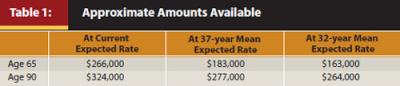
Table 1 sets out the range of approximate amounts available under each expected rate used in this paper, for ages 65 through 90. These figures are for home values equal to the pre-2009 HECM limit of $417,000 or greater. For home values greater or less than this limit, the available credit line amounts are essentially proportional. Thus, a home worth $300,000 would give rise to a credit line amount equal to about 300/417 = 72 percent of the amount set out in Table 1. Likewise, a home worth $600,000 would give rise to a credit line equal to about 600/417 = 144 percent of the amount set out in Table 1. When interest rates are higher, and hence amounts of credit available are lower, the effect on our calculations would be the same as lowering the home value, as described later in the paper.

Results

The essential result shown by our analysis is the substantial increase in cash flow survival probabilities that comes from reversing the conventional wisdom. This result holds true across a wide range of portfolio asset allocations, of home value to account value ratios, and of expected rates, and both with and without the use of safeguards similar to those described by Guyton (2004).

To best illustrate these results, we choose a specific example, described below. The results are a set of figures showing the cash flow survival probability for a range of 15 years to 30 years, under the set of assumptions described. There is a figure for each of three initial withdrawal rates, 5.0 percent, 6.0 percent, and 6.5 percent. The results in this example are indicative of both the qualitative and quantitative results of using a wide range of assumptions.

Before examining the results of the three strategies of using the reverse mortgage credit line, we first consider the results when the reverse mortgage credit line is not used at all. When the account is the only source of the retiree’s income, cash flow is not likely to survive very long if the initial withdrawal rate is much above the safemax level of 4 percent of the initial account value. Figure 1 shows the probabilities of cash flow survival for a range of initial withdrawal rates from 4 percent to 7 percent of the initial account value.

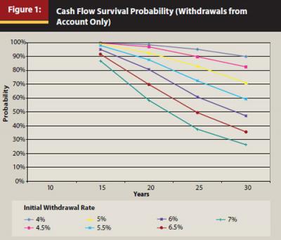
It is clear from Figure 1 that the probability of cash flow survival for 30 years falls below 90 percent when the initial withdrawal rate is 4.5 percent or more. Similarly, the probability of cash flow survival for 25 years falls below 90 percent when the initial withdrawal rate is 5 percent or more. At initial withdrawal rates of 5.5 percent or more, the cash flow survival probabilities fall to levels that should generate serious concern for the retirees whose life expectancies are greater than 25 years.

Results When the Reverse Mortgage Credit Line Is Added. We now illustrate the cash flow survival probabilities when the reverse mortgage credit line is used in addition to the account, in all three strategies. The illustrative example uses the following input data:

1. The initial account value is $800,000.¹⁵
2. The home value is equal to the pre-2009 HECM limit of $417,000. (We are not aware of any reverse mortgages currently available that provide loans based on home values higher than the HECM limit and provide the loans in the form of a credit line.)
3. The initial withdrawal rate is the primary variable used in our comparison of the three withdrawal strategies. We show results for initial withdrawal rates of 5.0 percent, 6.0 percent, and 6.5 percent.

In this example, we assume the retiree is age 65, and the resulting credit line available is approximately $266,000 in the initial year at the current expected rate and approximately $183,000 at the 37-year mean expected rate. In both the reverse-mortgage-last strategy and the coordinated strategy, the reverse mortgage credit line is established later in the 30-year sequence, so the amount available is greater.

In considering this example, it is important to note that the home value used to determine the reverse mortgage amount is approximately equal to 52 percent of the account value. If the home value were lower, or the account value were higher, the ratio of home value to account value would be lower; as a result, the effect of the reverse mortgage credit line on the probability of cash flow survival would also be lower. We show below a quantitative measure of the impact on our results of the ratio of home value to account value, both above and below this 52 percent ratio.

Results from Withdrawals Near the SafeMax Rate. Because the probability of cash flow survival for 30 years with initial withdrawal rates in the range of 4 percent to 4.5 percent is near 90 percent even without the use of the reverse mortgage, the use of the reverse mortgage credit line makes little difference. That is true irrespective of which of the three withdrawal strategies is used.

Results with a 5 Percent Initial Withdrawal Rate. The first initial withdrawal rate we examine, as we compare the three withdrawal strategies, is 5.0 percent. This initial withdrawal rate yields a significant increase in the annual withdrawal amounts over the safemax rate. In dollar terms, with an $800,000 initial account value, it reflects an $8,000 increase in initial annual withdrawal over the safemax amount. In percentage terms, it is an increase of 25 percent over the 4.0 percent safemax rate.

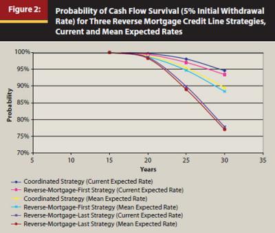
Figure 2 shows the probability of cash flow survival for the three withdrawal strategies, with a 5.0 percent initial withdrawal rate, for periods from 15 years to 30 years. It is clear from Figure 2 that, with a 5 percent initial withdrawal rate, the coordinated strategy and the reverse-mortgage-first strategy both result in cash flow survival probabilities significantly greater than the result of using the reverse-mortgage-last strategy. This is true with both the current expected rate and the mean expected rate. Specifically, the 30-year cash flow survival probability for both of the active strategies is approximately 95 percent with the current expected rate and approximately 90 percent with the mean expected rate. The cash flow survival probability for the reverse-mortgage-last strategy is less than 80 percent with both expected rates. Thus, the active and passive strategies result in a difference in the cash flow survival probabilities of 10 to 15 percentage points.

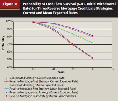
Results with a 6 Percent Initial Withdrawal Rate. We next take a larger jump in initial withdrawal rate in our comparison of the three withdrawal strategies by examining the results of a 6.0 percent rate.

This is almost 50 percent more than the safemax rate. In dollar terms, with an $800,000 initial account value, it reflects an increase of almost $16,000 in initial annual withdrawal over the safemax amount. This rate is such that, absent the reverse mortgage component, it results in a 60 percent probability of cash flow survival for 25 years and less than a 50 percent probability of cash flow survival for 30 years.

The results are shown in Figure 3. With the two active strategies, the 25-year cash flow survival probability is close to 90 percent with the current expected rate and 85 percent with the mean expected rate. The 30-year cash flow survival probability is over 80 percent with the current expected rate and over 70 percent with the mean expected rate. By contrast, the conventional (reverse-mortgage-last) strategy results in a 25-year cash flow survival probability of about 70 percent and a 30-year cash flow survival probability under 55 percent with both expected rates.

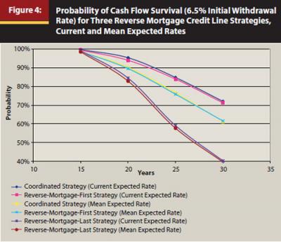
Results with a 6.5 Percent Initial Withdrawal Rate. The next initial withdrawal rate we examine is 6.5 percent. The results are shown in Figure 4. It is clear from Figure 4 that, with a 6.5 percent initial withdrawal rate, the 25-year cash flow survival probability, with either of the active strategies and the current expected rate, is below 90 percent. And the 30-year cash flow survival probability with either of the active strategies is barely above 70 percent. The reverse-mortgage-last strategy results in a 30-year cash flow survival probability of only 40 percent.

However, before hope is lost for initial withdrawal rates as high as 6.0 percent or 6.5 percent to have 90 percent or greater cash flow survival probability, we point out that there are at least three situations in which these initial withdrawal rates, and initial withdrawal rates even higher, can still result in cash flow survival probabilities of 90 percent or greater:

1. The first situation is where the ratio of home value to account value is higher than the ratio in our example. Holding the home value in our example constant, this situation would occur only where the account value is lower than in our example; in that case, the dollar amounts of the withdrawals would also be lower. This situation is illustrated in the next section.
2. The second situation is the obvious one, where there are higher investment returns on the portfolio than those used in our example. This situation is illustrated later in the paper.
3. The third situation is the one in which certain safeguards are used. The safeguards are described and illustrated later as well.

The Impact of the Ratio of Home Value to Account Value

Obviously, the greater the home value, the greater the increase it can provide to the cash flow survival probability. In the example we considered above, the ratio of initial home value to initial account value was approximately 52 percent.¹⁶ We now show how varying this ratio, as we hold the other parameters constant, alters the effect the different strategies have on cash flow survival probability. Specifically, we show in Figure 5, using an initial withdrawal rate of 6.5 percent, the 30-year cash flow survival probability as a function of the ratio of initial home value to initial account value.

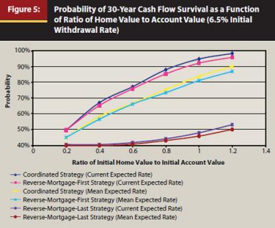
This figure shows a very high probability of cash flow survival when the ratio of home value to account value equals or exceeds 100 percent and one of the active strategies is used. For example, when the ratio is 100 percent, the conventional (reverse-mortgage-last) strategy still results in less than a 50 percent cash flow survival probability for 30 years, and the active strategies (at the current expected rate) result in a greater than 90 percent cash flow survival probability.

The active strategies show a sharp increase in the cash flow survival rate as the ratio of home value to account value increases, much more than does the conventional strategy. Thus, the higher the ratio, the greater the impact that comes from the active strategies as compared with the conventional strategy.

Because we hold the home value in our example constant at $417,000, ratios of home value to account value that exceed 52 percent require lower account values than the $800,000 value used above. Thus, for the calculations based on the 60 percent, 80 percent, 100 percent, and 120 percent ratios, we used account values of $695,000, $521,250, $417,000, and $347,500, respectively. Consequently, the initial withdrawal dollar amounts for the 6.5 percent initial withdrawal rate were $45,175, $33,881, $27,105, and $22,588 for those four account values, respectively.

The Impact of Higher Investment Returns

The cash flow survival probabilities determined with the use of the 32-year investment return data were noticeably higher than those determined with the use of the 37-year data. But the qualitative results were essentially the same—with each investment return data set, the active strategies yield substantially higher cash flow survival probabilities than the conventional (reverse-mortgage-last) strategy.

Figure 6 is indicative: the cash flow survival probabilities are shown for a 6.5 percent initial withdrawal rate for eight different situations. The upper four lines show the results of the coordinated strategy using the 32-year investment return data and the 37-year investment return data, each with the current expected rate and the applicable mean expected rate. It is obvious that the 32-year data yield greater cash flow survival probabilities. In fact, the 32-year data reflect investment returns sufficiently higher than the 37-year returns in that they bring the 30-year cash flow survival probability almost to 90 percent (and exceed 90 percent when the current home value limit of $625,500 is used instead of the pre-2009 limit of $417,000).

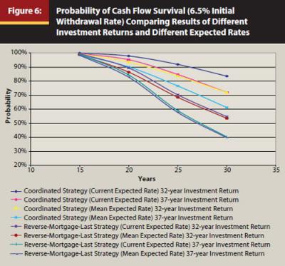
The lower four lines show the results of the conventional strategy, also using the 32-year data and the 37-year data, each with the current expected rate and the applicable mean expected rate. The reverse-mortgage-first lines have been omitted, simply for clarity. (As in the previous figures, the reverse-mortgage-first lines would be very close to the coordinated lines.) And again, the 32-year data yield greater cash flow survival probabilities.

It is noteworthy that the disparity between the results of the active strategies and the conventional strategy is somewhat greater in the case of the 37-year data than in the case of the 32-year data. This is evident in Figure 6, where, for example, the spread between the second and seventh lines is a bit greater than the spread between the first and fifth lines. This disparity also holds true with the other initial withdrawal rates. It suggests that the active strategies for using the reverse mortgage credit line are of somewhat greater value (relative to the conventional strategy) when investment returns are weak than when they are strong.

Effect of Certain Safeguards

The authors are aware of the innovative work of Guyton (2004) and Guyton and Klinger (2006) in the area of enhancing retirement income survival probabilities. Therefore, we thought it would be interesting to see how techniques similar to theirs could be used in conjunction with the reverse mortgage strategies we have studied. We focused on “withdrawal rule 2” plus the inflation decision rule, both of which are used by Guyton in the 2004 paper.

Under withdrawal rule 2, “there is no increase in withdrawals following a year in which the portfolio’s total investment return is negative, and there is no make-up for a missed increase in any subsequent year.”¹⁷ Under the inflation decision rule, “the maximum inflationary increase in any given year is 6 percent, and there is no make-up for a capped inflation adjustment in any subsequent year.” For simplicity, we call the combination of these two rules the “safeguards.” Incorporating the safeguards into our model significantly increases the cash flow survival probability with both the conventional strategy and the active strategies.

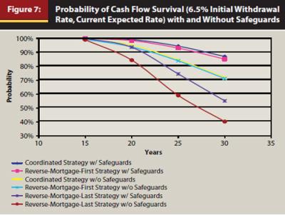
Figure 7 shows that, with a 6.5 percent initial withdrawal rate, the safeguards increase the 30-year cash flow survival probability when the active strategies are used from just above 70 percent to nearly 90 percent. (When the current home value limit of $625,500 is used instead of the pre-2009 limit of $417,000, the safeguards increase that probability from 80 percent to more than 90 percent.) The safeguards also increase the 30-year cash flow survival probability when the conventional strategy is used from about 40 percent to about 55 percent. Thus, the safeguards give approximately the same boost to the conventional strategy as to the active strategies. The results of incorporating the safeguards into the model at other initial withdrawal rates, and other expected rates, are similar.

Residual Net Worth

After reviewing the results of the calculations and analyses set out so far, the reader may ask whether the greater cash flow survival probabilities that result from the use of the active strategies come at the cost of lower residual net worth. We define the term “residual net worth” as the value of the retiree’s portfolio plus the equity in the retiree’s home at the end of the period in question. The equity in the home is the value of the home minus the cumulative reverse mortgage debt, including accrued interest.

This issue is important to the many retirees who, in addition to their primary concern for continuing cash flow throughout their retirement years, have a bequest motive or concern about late-in-life needs.

Our model includes a provision for calculating the residual net worth for each of the three strategies; it also calculates the differences of those quantities between each pair of strategies. When only the differences of the residual net worth are used, the value of the home subtracts out, leaving only the differences of the account values and the differences in the accrued reverse mortgage debt. We define this as a positive difference if, at the end of any trial, the residual net worth of the coordinated strategy exceeds the residual net worth of the reverse-mortgage-last strategy.¹⁸

When the percentage of trials with positive differences is greater than 50 percent, it indicates that the residual net worth is more likely than not to be higher with the coordinated strategy than with the reverse-mortgage-last strategy.

Without setting out a detailed display of these results, we note that, for initial withdrawal rates from 4.5 percent through 7.0 percent, we find positive differences in 67 percent to 75 percent of the trials. Thus, in this range of initial withdrawal rates, the choice of an active strategy rather than the conventional strategy is between two and three times more likely to result in a positive difference in residual net worth than in a negative difference.

Conclusions

We have considered retirement income in the classic mode of constant purchasing power (except where the safeguards are invoked) over periods of up to 30 years. The income sources we have considered consist of a securities portfolio plus withdrawals from home equity by means of a reverse mortgage credit line.

We have focused on cases in which the initial withdrawal rate exceeds the so-called safemax rate of approximately 4 percent of the initial portfolio value. In those cases, particularly in the range of initial withdrawal rates between 5 percent and 6.5 percent, we have found substantially greater cash flow survival probabilities when the reverse mortgage credit line is used in either of two active strategies rather than in the conventional, passive, strategy as a last resort. We have also found that use of these active strategies is likely to result in a higher residual net worth after 30 years than the use of the conventional strategy.

Endnotes

1. Brandon, Emily. 2011. “How to Retire on Social Security Alone.” U.S. News & World Report (May 16).
2. Because the retirement accounts are generally invested in portfolios of securities, and because our analysis is based on the behavior of securities portfolios, the terms “account” and “portfolio” can be considered interchangeable in this context. In the case of a retiree taking withdrawals from a pre-tax account, such as an IRA or a 401(k) plan, the retiree’s expenses will include his or her income taxes.
3. See, for example: Bengen, William. 2006. “Sustainable Withdrawals.” In Retirement Income Redesigned, edited by Harold Evensky and Deena B. Katz. New York: Bloomberg Press.
4. There exist a small number of financial products similar but not identical to reverse mortgages. These include, among others, “NestWorth” and “FirstREX.” The analysis and computations set out in this article are based explicitly on reverse mortgages. However, the results, at least qualitatively, also apply in situations in which other such financial products are used to supplement withdrawals from the account.
5. See, for example: Lieber, Ron. 2011. “Reverse Mortgages Here to Stay.” New York Times (June 25): “[Reverse mortgages] will almost certainly become a necessary last resort for a nation full of increasingly strapped people.” See, also: Quinn, Jane Bryant. 2011. “Picking the Right Options.” AARP Bulletin (May): “And don’t take a reverse mortgage in your 60s. Save these loans as a last resort, for money in your older age.” As another example, see: Osterland, Andrew. 2011. “The Retirement Tool Advisors Love to Hate.” Investment News (April 11–15): “‘Your home should be the absolutely last asset you tap,’ said Joseph Duran, chief executive of United Capital Financial Partners Inc.” See also: Pond, Jonathan. 2010. “Retired and Loving It!” AARP Magazine (May/June): “You know your money will last when...you won’t need a reverse mortgage until age 80 or later. These costly deals are best viewed as a late-in-life trump card to keep you in your home.”
6. There is a minor modification in certain cases when the investment performance was positive: if the dollar amount of the account’s positive return was less than the withdrawal amount scheduled for the next year, only the amount of the positive performance is taken from the account, and the remaining portion of the scheduled withdrawal amount is taken from the credit line. Also, of course, if the investment performance was negative but the reverse mortgage credit line has already been exhausted, the entire withdrawal will come from the account.
7. The algorithm described here, with its embodiment in a computer-based system for advising retirees on withdrawal amounts and sources, is the subject of a patent issued to the authors November 8, 2011.
8. We recognize that inflation figures for any year tend to relate to those of the preceding years, rather than vary stochastically. We plan to further refine our model and our analysis to reflect that fact.
9. It is worth noting that in some of the repetitions the portfolio survives with very substantial value at the end of the 30-year period, and in others the portfolio survives with very little value at the end of the period.
10. Bengen, ibid.
11. There are many sources of information on reverse mortgages. See, for example, http://portal.hud.gov/hudportal/HUD?src=/program_offices/housing/sfh/hecm/hec, which includes, among other information, a link to the AARP website.
12. FHA Mortgagee Letter 2011-39, December 2, 2011.
13. These factors can be found at: http://portal.hud.gov/hudportal/HUD?src=/program_offices/housing/sfh/hecm/hecmhomelenders.
14. Because the expected rate appears only once in each 30-year trial, our model does not Monte Carlo simulate the expected rate. By means of a set of tests, we have determined that there is no significant difference between the cash flow survival probability results of using a single expected rate throughout a series of trials and the results of Monte Carlo simulating the expected rate throughout the same series with a normal distribution around the same expected rate.
    Another parameter relevant to the reverse mortgage, but less directly relevant to cash flow, is the so-called “current rate.” The current rate is determined each year and is the short-term interest rate (typically the one-year Treasury rate or the one-year Libor rate). It is used every year for two purposes: (1) it determines the rate at which amounts already drawn from the credit line accrue interest that year, and (2) it determines the increase in the amount still available from the portion of the credit line not yet drawn. The second purpose does affect cash flow to the retiree. This parameter is Monte Carlo simulated in our model.
15. This value, although just part of an illustrative example, is chosen because it is very close to the average value of the “investable and disposable assets” held by the members of “Group 3” (those who have a “paid planner and a comprehensive written plan”), age 65 and over, as described in the 2008 FPA and Ameriprise Value of Financial Planning Study: Consumer Attitudes and Behaviors in a Changing Economy, conducted by Harris Interactive. (The average is computed without the one outlier who reported investable and disposable assets of $20 million or more.)
16. At least through December 31, 2012, $625,500 is the maximum home value that can be taken into account in any reverse mortgage that can be drawn upon in the form of a credit line. Therefore, home values larger than that limit, although theoretically increasing the ratio of home value to account value, in practice do not increase the ratio.
17. We could not use the modified form of the withdrawal rule described in the 2006 work, because that rule involves the withdrawal rate at the time of each year’s withdrawal. That rate is equal to the amount of the withdrawal divided by the value of the account. Our three-spreadsheet model has the withdrawal in any given year coming from different sources on the different spreadsheets, and hence the value of the account in any given year (except the first year) generally differs among the three spreadsheets. Therefore, if we were to use the modified withdrawal rule, the amounts of the withdrawals (in some years, and hence cumulatively) could be different among the three strategies; this would be inconsistent with our approach to the comparison of the three strategies, under which the withdrawal amount is the same for each strategy.
18. It is important to note also that the range of likely outcomes of the difference of residual net worth, at the end of 30 years, is extremely wide.

References

Guyton, Jonathan. 2004. “Decision Rules and Portfolio Management for Retirees: Is the ‘Safe’ Initial Withdrawal Rate Too Safe?” Journal of Financial Planning (October): 54–62.

Guyton, Jonathan and William Klinger. 2006. “Decision Rules and Maximum Initial Withdrawal Rates.” Journal of Financial Planning (March): 48–58.