Journal of Financial Planning: February 2012
Jerry A. Miccolis, CFA, CFP®, FCAS (miccolis@brintoneaton.com), is a principal and the chief investment officer at Brinton Eaton, a wealth management firm in Madison, New Jersey, as well as a portfolio manager for The Giralda Fund. He co-wrote Asset Allocation For Dummies® (Wiley 2009) and numerous works on enterprise risk management.
Marina Goodman, CFP® (goodman@brintoneaton.com), is an investment strategist at Brinton Eaton and a portfolio manager for The Giralda Fund. She has been working to bridge the gap between research and practice in improving the portfolio optimization process, and has written numerous articles on the subject.
Executive Summary
- The best-designed asset allocation and rebalancing systems are not infallible—they were not designed to meet every market circumstance. Something else is needed when the core assumptions of modern portfolio theory (MPT) are violated.
- Dynamic asset allocation (DAA) is a response to those times when MPT’s key assumptions need to change.
- Rebalancing, which is designed to exploit mean reversion among asset-class returns, needs to be taken to the next level.
- A particular example of DAA, momentum-based moving average (MA) strategies, represents a more proactive means of achieving the goals of rebalancing. A specific application of an MA strategy is illustrated.
- DAA, in combination with “modernized” MPT (discussed in our January 2012 JFP article) and tail-risk hedging (when all else fails), collectively form the vanguard of the next generation of investment risk management.
The repeated stresses the capital markets have experienced over the past decade have caused many financial planners to question all they thought they knew about investment management. Modern portfolio theory (MPT) and its core component strategies, asset allocation and rebalancing—indeed, any investment strategy not involving cash in mattresses—came under attack. After experiencing significant wealth destruction more than once in the past 10 years, even planners who acknowledge that these core strategies still form the bedrock of prudent investment management are asking themselves: are we missing something?
The best-designed MPT/asset allocation/rebalancing system is not infallible. As discussed in our recent Journal of Financial Planning article (Miccolis and Goodman 2012), MPT rests on certain fundamental assumptions. For example, rebalancing depends on mean reversion on the part of asset-class returns. What happens when mean reversion takes a holiday, and markets suffer protracted declines? What can we do when our MPT assumptions as a whole suddenly, inexplicably, and dramatically change?
This article explores a robust way to deal with these eventualities. We will describe a systematic method to make your client portfolios more proactive in their response to market volatility. In fact, this approach can be viewed as a way to exploit that volatility.
To set the stage, let’s first take a closer look at the traditional approach to exploiting market volatility—portfolio rebalancing.
Rebalancing Revisited
Rebalancing is really nothing more than keeping your portfolio true to its intended asset allocation. Over time, asset classes tend to grow at different rates. Without rebalancing, this may cause the overall risk profile of the portfolio to change substantially, likely getting riskier as higher-risk/higher-return asset classes outgrow their counterparts. Worse, this tends to make the portfolio drift off the efficient frontier and occupy the inefficient interior of risk/return space.
Rebalancing restores order by trimming the leaders among the asset classes and redeploying the proceeds into the laggards. This is, therefore, a risk management device, one that attempts to keep the portfolio hugging the efficient frontier. By doing so, it allows portfolios to occupy a more efficient region of risk/return space than they otherwise could. In effect, then, it shifts the entire frontier upward relative to a world in which rebalancing is not performed, allowing the portfolio manager to capture extra return for no increase in risk—the closest thing to a free lunch in investing. The mathematics behind this “rebalancing benefit” can be found in an excellent paper by Bernstein and Wilkinson (1997).
What is the essence that makes the rebalancing benefit work? Mean reversion. Specifically, mean reversion among asset classes that don’t mean revert on the same schedule. (An illustrated example of this is provided in Miccolis and Goodman 2012.)
Mean reversion refers to the tendency for assets, once they’ve ventured “too far” from their long-term trend line, to change direction and revert back toward their trend line. Momentum and mean reversion can be seen as opposite sides of the same coin. Momentum continues until it runs out of steam, then mean reversion takes over as the driving force, leading to momentum in the other direction. Rebalancing allows the portfolio to enjoy an asset class’s upward momentum, and then take some winnings off the table before mean reversion kicks in. It also prompts you to “double down” on an asset class whose mean reversion is about to propel it upward. When it is working properly, rebalancing is a systematic way to buy low and sell high, repeatedly.
One way to rebalance is to do so on a fixed calendar schedule. We believe a more opportunistic approach is better—one based on tolerance bands. Under this approach, you rebalance only if and when an asset class’s allocation drifts beyond its target by more than a certain threshold, say plus or minus two percentage points. A very nice discussion of tolerance-based rebalancing is offered by Daryanani (2008).
Whether calendar-based or tolerance-based, rebalancing is a way to exploit momentum/mean reversion without having to venture a guess as to when the directional changes might occur. It is the passive, reactive approach. Some might call it the naïve approach. It doesn’t always get the timing right, but it’s close enough—often enough—to pay benefits over the long run.
Here’s a way to visualize what goes on. Think of each asset as tethered to its long-term trend line by a leash. The asset can roam freely from its trend line to a degree, but if it strays too far, the leash gets pulled taut and snaps the asset back in the opposite direction. Tolerance-based rebalancing is implicitly assuming that the length of this leash is a predetermined constant. When an asset’s allocation has reached this threshold, you are assuming that momentum is near its end, and mean reversion is about to take over.
Although this leash analogy may be evocative, in the real world of asset behavior, the leash is of indeterminate—and changing—length and elasticity. How do you deal with that? Additionally, what happens when normally uncorrelated asset classes start behaving similarly—when they no longer mean revert on different schedules? Rebalancing will have nothing to do if all asset classes suffer similar declines at the same time. What then?
Enter dynamic asset allocation (DAA). DAA holds the promise of being able to take rebalancing to the next level. It allows us to make more informed choices about whether we want to rebalance or wait and let momentum run. It can also tell us if it is time to reconsider our target asset allocations altogether.
Taking Rebalancing to the Next Level
First, let us reaffirm our faith in modern portfolio theory (suitably modernized, as discussed in Miccolis and Goodman 2012). Although MPT is as useful as ever, the market behavior of the past decade has clearly shown financial planners the dangers of using static assumptions and allocations.
Helping our clients maintain their lifestyle for decades into the future requires us to take a long-term view. However, having a long-term view does not require us to be blind to what is currently occurring. After all, how were our portfolio allocations developed in the first place? Setting a target asset allocation starts with making assumptions about the economy and different segments of the market. These assumptions then lead to estimates of the risk, return, and relationships of different assets—the three inputs of an MPT model. Subsequently, an efficient frontier of optimal portfolios is derived, and the specific portfolios to be used for various categories of clients are selected from the frontier.
But what if economic and market conditions change? Why shouldn’t the MPT assumptions/inputs change? How would you know that things have changed enough to warrant a significant shift in your assumptions? And how would you then change your assumptions? Even if you just use historical data to forecast your asset classes’ returns, risk, and relationships, these will change over time as well. Lastly, when should you modify the allocations in the portfolios to reflect the new assumptions?
Talking about changing allocations makes some investors nervous. Investment managers pride themselves on keeping their eye on the long term and not being swayed by the daily market hoopla. Is a change in the portfolio a strategic decision based on long-term predictions or a tactical adjustment based on the crisis du jour?
DAA bridges the divide between the long-term strategic and the short-term tactical. DAA is a systematic, proactive, forward-looking approach to asset allocation and rebalancing. With DAA, you are looking for early warning indicators that can reliably tip you off when the fundamental assumptions you used in creating the optimal efficient frontier have changed or are likely to change soon. You then make tweaks to your MPT inputs, promptly re-optimize the efficient frontier accordingly, and determine your new target allocation percentages.
The challenge is to find economic and/or market signals that are both reliable and timely. There are two broad categories of signals: external to the market (for example, leading economic indicators), and internal (movements in the asset class itself). In this article, we briefly discuss external signals immediately below, and then spend a good bit of time on one category of internal signals we have found especially useful.
One part of DAA is determining which elements of myriad economic and market data can serve as early warning indicators to alert you when your key assumptions/inputs need to change. Picerno (2010) lists numerous indicators. Examples of common economic indicators are inflation rate, unemployment rate, and gross domestic product (GDP) growth. Market-based signals include price/earnings ratios, book/market ratios, volatility, interest-rate levels and term structure, credit spreads, and money flows. The full list of external indicators is virtually inexhaustible and beyond the scope of this article.
When the economic landscape shifts sufficiently to cause you to change the assumptions you used in determining the optimal asset allocation, you re-estimate the efficient frontier based on your revised assumptions. The next question is: when do you implement the new asset allocations implied by the new efficient frontier? There are numerous examples of investment managers being right about their predictions but wrong about their timing, causing them to lose clients before their predictions had a chance to come true. Therefore it is crucial to determine when it is more likely your predictions will become reality. For that, it is helpful to look at the markets’ internal signals.
These internal signals can also be used independently of external signals. They are very valuable in their own right. Before we examine a particularly useful class of internal signals, it is instructive to dig deeper into what makes these types of signals tick—momentum.
Momentum and Moving Averages—a Primer
Numerous market metrics can be used to check the pulse of a market and identify trends. The metric we will focus on here is momentum—the tendency of assets going in a particular direction to continue to move in the same direction. The most common way to measure momentum is by calculating a moving average (MA).
Some investors may view MA strategies with great suspicion, as they are closely associated with ultra-short-term technical analysis, market timing, and everything that is anathema to pure, strategic, long-term investing (see DAA sidebar). As will be shown, though, these MA strategies are quite flexible and can be constructed to be as short term or long term as desired.
Using moving averages to extract information is not a new concept; it is borrowed from electrical engineering, specifically the field of signal processing. The capital markets can be viewed as emitting numerous signals. Some are “true” signals—valuable data that give you an indication of what is happening now and what will likely happen in the future. Most are “false” signals—white noise, static, distracting din. The goal of signal processing is to develop the right filter, or set of filters, to allow the true signals to get through and eliminate as much static as possible. In this article, we will look at only one type of market signal—momentum—and focus on one way it can be filtered—via its moving average.
Just as the crux of investment management is balancing the trade-off between risk and return, the crux of signal processing is managing the trade-off between “stability” and “responsiveness.”
To see how this concept applies to markets, consider the graphs in Figure 1. The top graph shows the S&P 500 Stock Index along with its 250-day MA, and the bottom graph shows the same index with its 50-day MA.
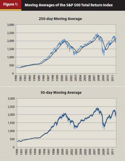
Note how the 250-day MA is quite smooth and unperturbed except by the longest and most pronounced overall movements in the index. A strategy based on this MA would have had very few trading signals over the last 20 years. These features come at a price. Note how the 250-day MA peaks well after the index has already suffered a decline, and it troughs well after the index has already rebounded. Also, numerous substantial declines and increases in the market are not captured by the shape of the 250-day MA. A 250-day MA would be considered a “stable” filter. Its advantage is that it eliminates almost all the static and therefore provides relatively few trading signals. Its disadvantage is it also eliminates some important true signals and is particularly vulnerable during the major inflection points in the market.
Now consider the 50-day MA. It is quite jagged and looks like only a slightly smoother version of the index itself. Using this MA for an investment strategy would cause you to trade far more frequently, often reversing trades within short periods. However, note that its peaks are close to the peaks for the index itself, and its troughs are close to the index’s troughs. A 50-day MA would be considered a “responsive” strategy. On the one hand, it lets in much more static, meaning it would cause you to do many more trades that it would soon tell you to reverse. However, its great benefit is in how it alerts you earlier to major inflection points in the market—the beginning of protracted bear and bull markets—than the 250-day MA.
The examples above demonstrate how the degree of stability and responsiveness of an MA filter can be varied just by changing the period over which it is measured. A longer period will result in a more stable filter. Therefore, although MAs are favorite technical indicators for very short-term investors, they can also be used by the most technical-averse, long-term investor.
The degree of stability versus responsiveness of an MA signal need not be static and may change based on market conditions. For example, if there has been a protracted bull market, and economic indicators are showing there will likely be a decline, an adviser may want to make the MA filter more responsive so it will show sooner when to get out. An adviser would also want to do this after a protracted bear market when the market is starting to give positive signals. On the other hand, when it looks like the market will be trending in a certain direction for a while, one is better off with a more stable filter.
The stability of the filter can be adjusted manually based on manager discretion, or it can change dynamically based on market behavior. For example, when there is an increase in volatility, there is often also a decrease in returns. It doesn’t always mean a decrease in return, so you don’t necessarily want to exit the asset class, but you do want to be more careful, more responsive. You may have a formula that calculates the current level of asset volatility and uses it to dynamically adjust the MA period, thereby making it more or less responsive automatically.
Types of Momentum Strategies
The number of investment strategies using momentum and moving averages is limited only by your imagination. Here we describe a few common approaches. The simplest strategy is to have a fixed period over which the MA is measured and to compare the index versus its MA. If the index is above its MA, then you stay invested in the index; otherwise you get out. The S&P Commodity Trends Indicator referenced by Miccolis and Goodman (2012) is an example of this approach, applied separately to each of the component commodities in the index.
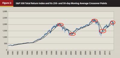
Another common strategy uses two MAs—one over a shorter period and one over a longer period. Instead of comparing the index itself to the MA, you invest in the asset if the shorter-period MA is greater than the longer-period MA. This is called a moving-average-crossover (MAC) strategy. Figure 2 shows this approach applied to the S&P 500 Index, using the same 250-day and 50-day MAs as before. Note how the major crossover points (in red) appear to be promising signals of turning points in the underlying index.
A third, less common strategy is to look at the trend in (the first derivative of) the MA. When the MA is increasing, one invests in the asset; when it is decreasing, one stays out.
Each of the above strategies can be enhanced substantially by making the MA period (the width of the MA window) dynamic based on external and internal market signals. The various strategies can also be used in tandem.
We have developed and tested dozens of types of momentum strategies. The number of possible strategies is virtually unlimited. In many ways the strategies we tested performed similarly—they all gave a signal to get out during bear markets and to get in during bull markets. Because momentum strategies rely on actual past movements in the asset, they are reactive instead of truly proactive. They will never get out at the top of the market or get in at the bottom. In order to do that you would need a predictive model that is 100 percent correct, which is, of course, unattainable. Therefore, all momentum models are vulnerable, in varying degrees, when the market is at an inflection point or is vacillating.
It is not too difficult to design a strategy that outperforms a buy-and-hold strategy over a sufficiently long investment horizon. The example in Figure 2 alone suggests how easy that would be. Other examples can be found in the literature.1 However, many of the strategies also underperformed for extended periods within the long horizon, which we found unacceptable. An ideal strategy would allow one to participate close to 100 percent of the time when the asset increased in value and avert significant losses. Limiting losses too extensively may cause one to miss too many of the gains, defeating the purpose.
Testing and Results
We asked the following questions when evaluating the candidate strategies: Does it materially and consistently outperform a buy-and-hold strategy? What is its lowest rolling annual return? What is its maximum drawdown? Under what conditions is the strategy most likely to underperform, outperform, or keep pace with the buy-and-hold benchmark?
What we found was that no momentum strategy was perfect, but several had unique strengths under different market circumstances. One strategy was very stable but was relatively late to get in and out. Another strategy did not outperform consistently but had more reliable signals as to when to get back into the market. A third strategy gave quite early indications of market inflection points under certain extreme conditions.
A breakthrough occurred when we realized that, instead of needing to select a single strategy, we could construct a “team” of them—a team on which each strategy had a role to play precisely under the circumstances when it is most likely to succeed. The “switches” to tell us when to move from one strategy to another were quite intuitive and easy to determine. We also implemented an additional overall filter to make the signals more stable.
In testing the model’s structure, we used both the S&P 500 Index and the individual equity sectors that constitute it. The S&P 500 Index gave us a much longer history than the individual sectors, so that we could better test how well our model would work under a greater variety of market conditions. This reduced the possibility that a particular strategy or set of parameters would work only over a specific period or type of market. Using the 10 equity sectors allowed us to develop a sector rotation strategy—when one sector got an “out” signal, the strategy had other sectors over which to redeploy the proceeds. The significance of this feature for a portfolio will be demonstrated shortly.
We optimized the parameters using only some of the available historical data and tested the model using a different set of historical “out-of-sample” data. This allowed us to test how the strategy would have done without gambling our clients’ money. We did, however, use our own funds to test it in real time. We even used the parameters optimized for one sector in calculating the performance of another sector, just to see how well the model would stand up to having suboptimal parameters. The overall performance of the model with these suboptimal parameters was similar to a buy-and-hold strategy but with significantly lower maximum drawdown—an encouraging sign of the strategy’s robustness. We did everything we could to make sure that the model would work in the future and was not a product of back-testing or data mining.
Figure 3 shows an example of applying our multi-layered momentum strategy to the Consumer Discretionary sector. We assumed that when we received an “out” signal we would go to cash, which we assumed earned 0 percent. Figure 3 includes a graph over the entire period 2/1991–5/2011, which includes the back-tested period (2/1991–12/2007) and the out-of-sample period (1/2008–5/2011) as well as graphs that show performance during the different types of markets over four subsets of that period.
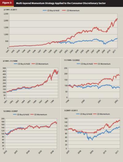
As can be seen, the strategy amply participates during bull markets but avoids significant losses during bear markets. The result is a threefold improvement in cumulative return over the full period 2/1991 to 5/2011.
Although these strategies can be used in isolation for individual sectors and asset classes, more of their power can be unleashed within the context of a rotation strategy among different market segments. These market segments can be as broad or granular as desired. They can be used at the broad asset-class level to help determine which asset classes to invest in, and within those asset classes to determine which sectors or securities to rotate among. We created strategies for each of the S&P equity sectors and combined them to create a dynamic, momentum-based, sector rotation strategy. The results are in Figure 4.
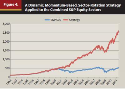
A breakdown of results by period looks similar to the graphs for Consumer Discretionary in Figure 3. Of particular note is the strategy’s performance during the 2000–2002 bear market when it experienced a healthy increase. Because the market’s decline was largely the result of a single sector, the sector rotation strategy was able to withdraw from the most affected sectors and redeploy funds to the other sectors that performed well. Note also that the only period of significant decline, the 20 percent drop in the fourth quarter of 2008, is considerably less than the roughly 50 percent decline in the S&P 500 over that period. The strategy was not as effective at minimizing losses during this period as during the 2000–2002 period because the more recent decline happened quite suddenly, whereas in 2000–2002 it occurred at a slower pace over a protracted period, thereby giving the momentum signals ample time to react. The strategy could be tweaked to make the drawdown in any period as small as desired on a back-tested basis, but that would come at the cost of having the strategy not perform as well overall. And because we have also done other work to address periods as unique as late 2008,2 we were comfortable with the strategy as is.
It should be clear that momentum strategies are not designed to predict turning points; they are designed simply to identify trends as promptly as possible after they develop and to suggest appropriate responses.
Is This All We Need?
Momentum/MA strategies do not supplant traditional asset allocation and rebalancing. All these strategies provide are “in” and “out” signals. You still need asset allocation to determine the optimal target allocation. And rebalancing is still needed to maintain the target allocation and take advantage of volatile diversified assets. Momentum/MA strategies are designed to help when asset allocation/rebalancing strategies are most vulnerable—during periods of protracted market decline. Beyond that, it is important to remember that MA algorithms are but one class of strategies in the broader array of portfolio management approaches under the umbrella of DAA.
Endnotes
- Faber, Mebane. 2007. “A Quantitative Approach to Tactical Asset Allocation.” Journal of Wealth Management (Spring); Wong, Theodore. 2009. “Moving Average: Holy Grail or Fairy Tale.” Advisor Perspectives (June 16, June 30, and July 28).
- As promising as DAA approaches may be, they are, like MPT itself, not infallible. There will be times when market misbehavior conspires to upset even the most robust, proactive portfolios. There inevitably will be the next “black swan” event. During those events, when nothing else works, your portfolio needs an explicit safety net. As mentioned, we also have done much work in this area—tail-risk hedging—and plan to report on it shortly.
References
Bernstein, William J., and David Wilkinson. 1997. “Diversification, Rebalancing, and the Geometric Mean Frontier.” Abstract #53503 at www.SSRN.com.
Daryanani, Gobind. 2008. “Opportunistic Rebalancing: A New Paradigm for Wealth Managers.” Journal of Financial Planning (January).
Miccolis, Jerry A., and Marina Goodman. 2012. “Next Generation Investment Risk Management: Putting the ‘Modern’ Back in Modern Portfolio Theory.” Journal of Financial Planning (January).
Picerno, James. 2010. Dynamic Asset Allocation: Modern Portfolio Theory Updated for the Smart Investor. New York: Bloomberg Press.
Sidebar:
DAA: Strategic? Tactical? Market Timing?
“Tactical” asset allocation has traditionally been distrusted by long-term strategic investors, which we consider ourselves. And “market timing” is considered downright heretical. Well, doesn’t dynamic asset allocation (DAA) seem awfully tactical? And doesn’t it look like market timing? How does one reconcile those views?
A Continuum. Although we firmly believe asset allocation should be strategic and long term, we have also always believed that it is only as good as the assumptions on which it rests. That’s why we have always revisited the allocations we have in place for our clients on a regular basis and tweaked those allocations when appropriate. Assumptions can and do change (for example, valuation does influence expected asset-class returns, volatility and correlations do vary over time, and economies do run in cycles); it is imprudent to pretend otherwise. DAA is simply a structurally sound way to continually test your foundational assumptions and nimbly make adjustments as appropriate.
DAA takes what we have always done and does it in a more timely manner. Viewed in this way, there is no real distinction between tactical and strategic—it is more of a continuum. The more frequently you check your assumptions and make strategic shifts when you should, the more tactical your behavior may appear.
Market Timing. As we see it, market timing is an attempt to outsmart the markets—a way to express your view of where markets are heading next by betting your client’s portfolio on it. We don’t think anyone is smart enough to get these guesses right consistently enough to fashion an investment strategy around it. Market timing purports to replace a financial/economic theoretical framework with gut instinct. DAA, on the other hand, does not repudiate the financial/economic principles that are the bedrock of MPT; it just recognizes more of them than traditional MPT does (for example, valuation matters, expected returns move in cycles, volatility is itself volatile, and asset-class relationships are dynamic). Unlike market timing, DAA is not a get-rich-quick scheme; it is a fundamentally sound, fully realized, not-get-poor-quick risk-management approach.
Bottom Line. Call it what you will, DAA is sound stewardship of client assets, in our view. In the end, our fiduciary duty to our clients trumps all labels.