Journal of Financial Planning: December 2013
Executive Summary
- This paper presents two important innovations that will help financial planners improve the spending and asset allocation decisions of their clients in retirement.
- The current prevalent approach of using a deterministic planning horizon (assuming a single death age) to assess sustainability risk often misrepresents the actual risk of running out of money in retirement.
- This paper proposes a simple way to measure sustainability risk—mortality-adjusting—that accounts for the joint occurrence of being alive and running out of money.
- Different assumptions regarding the age of death of a client leads to very different assessments of retirement sustainability risk.
- Results show the discrepancy in assessed sustainability risk computed using these different deterministic planning horizons, relative to the mortality-adjusting approach, to be quite large.
- Findings can help planners more accurately represent sustainability risk, thereby increasing the value they deliver to their retired clients.
Grant Gardner, Ph.D., is a consultant at Gardner Financial Economics who advises Russell Investments on investment issues related to retirement. He was formerly a director of research at Russell Investments. Email HERE.
Sam Pittman, Ph.D., is a senior researcher at Russell Investments, primarily focusing on allocation solutions for retired investors. He is engaged in the research of retirement sustainability and asset liability modeling, which supports Russell’s private client practitioner and defined contribution plan clients. Email HERE.
Most retired investors want to maximize retirement income while limiting the risk of running out of money before they die. Financial planners call this sustainability risk. Retirees develop spending plans based on their tolerances for sustainability risk. Additionally, financial planners select investment strategies to fund spending plans based on sustainability risk. Because such important decisions are based on sustainability risk, an accurate assessment is critical to the development and implementation of a retirement plan.
To evaluate sustainability risk, planners typically select a horizon that is based on a conservative estimate of a client’s time of death, such as the age to which the client has only a 10 percent chance of living. Next, planners evaluate the risk of running out of money before this horizon, taking into account uncertain investment returns, often using Monte Carlo simulations to generate estimates.
Although the prevalent way to measure sustainability risk is to evaluate running out of money before a selected plan horizon1, the actual risk faced by a retiree depends on two events: running out of money and being alive when money runs out. Hence, there are two sources of uncertainty that determine sustainability risk: (1) uncertainty regarding the investor’s lifespan and (2) investment return uncertainty. The prevalent approach captures investment return uncertainty, but fails to represent lifespan uncertainty.
Consider the following example. An adviser tells a single, 65-year-old male client that after evaluating his spending plan with her recommended investment strategy, he has a 30 percent chance of running out of money in retirement. The client says, “I can’t live with a 30 percent chance of running out of money; I want to lower my spending.” The client lowers his spending. What the adviser did not tell the client was that she assumed a death age of 99 years old, which is the 95th percentile life span of a 65-year-old male.
What’s wrong with the advice to reduce spending? The adviser significantly overstated the chance that the client would run out of money in retirement. If the client has only a 5 percent chance of living to age 99 and a 70 percent chance of having wealth if he lives to age 99, his odds of dying penniless are much less than 30 percent. Nonetheless, the client decided to reduce his spending, forgoing a better lifestyle in retirement because of a faulty risk assessment.
When lifespan uncertainty is ignored, the assessed sustainability risk depends on the choice of the planning horizon. Assuming longer planning horizons or higher death ages will make a plan look riskier. For example, assessing the chance of running out of money up until age 90 versus age 100 will lead to different risk assessments.
Because spending decisions and investment decisions are based on sustainability risk, these choices may be made incorrectly if sustainability risk is misestimated, as in the previous example. This concern is addressed in this paper where two important innovations to improve the consistency of advice are made. First, the analysis demonstrates that the prevalent approach of using a deterministic planning horizon (single assumed death age) leads to advice that is based on incorrect assessments of risk. Second, a simple way to measure sustainability risk that accounts for the joint occurrence of being alive and running out of money, which is called mortality-adjusting, is described. Mortality-adjusting removes the dependence of sustainability risk on the planning horizon. This approach acknowledges the possibility of all death ages in a manner that is consistent with the probabilities in actuarial life tables.2
A Model of a Retiree’s Investment and Spending Decisions
To illustrate the problems resulting from using a deterministic planning horizon, a simple model of a retiree’s investment and spending decisions was constructed. If one assumes a deterministic planning horizon, a retired investor must choose a spending plan up to that horizon and an investment strategy to fund that spending.
The spending plan consists of a sequence of desired spending amounts each year. The sequence of desired spending could be fixed or based on some rule that includes annual variations due to changing needs or adjustments for inflation (see Guyton (2004), Guyton and Klinger (2006), and Blanchett, Kowara, and Chen (2012) for alternative spending strategies). In the model, spending occurs after market returns at the end of the year. The remaining wealth is then invested according to the investment strategy.
It was assumed in this paper that portfolio returns generated by the chosen investment strategy are uncertain. Therefore, the investor may not be able to fund all of his or her desired spending. The relationship between actual and desired retirement spending follows a simple rule: if the investor’s portfolio at the end of the period is greater or equal to desired spending, then he or she spends the desired amount. If the portfolio is less than desired spending, the investor consumes all of his or her remaining wealth. When wealth is reduced to zero, there is no future investing or spending. The investor has run out of money.
The investment strategy that funds the spending plan could be a simple fixed-mix allocation rebalanced periodically, such as a 40/60 percent mix of equities and fixed income, or it could be more complex. Examples of complex strategies are pre-determined but changing allocations (often called glide paths) and dynamic strategies where the allocation is a function of wealth, past returns, or some other variables (Fan and Gardner 2012; Fan, Murray, and Pittman 2013).
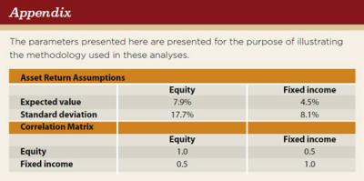
In the discussion and examples presented here, it was assumed that asset returns are random variables with a known probability distribution. Because each asset’s return is random, the portfolio return is also random with a probability distribution that depends on the return probability distributions of the individual assets and the investment strategy. Monte Carlo simulation was used (return assumptions shown in the appendix were used to simulate asset returns).
A retirement strategy, consisting of a spending plan and an investment strategy to fund it, is sustained if all of the desired retirement spending occurs and the investor does not run out of money prior to the planning horizon. Generally, whether or not a retirement strategy will be sustained is uncertain. It is this uncertainty that causes sustainability risk. (Retirees face a variety of unknowns beyond the discussion of investment return uncertainty, such as health care expenses.)
Sustainability risk was measured in terms of expected shortfall.3 Shortfall is a measure of the magnitude of failure in sustainability. It is defined as the sum of the desired spending that is not available because the portfolio is exhausted before death. For example, if a retiree who dies at age 85 exhausts his portfolio after his 83rd birthday, his shortfall will equal the sum of his desired spending in his 84th and 85th years of life.
Even in the case where an investor’s lifespan is deterministic, the value of shortfall at the end of life is uncertain because the return on the portfolio is a random variable. Expected shortfall is the average shortfall across all potential investment return paths. Expected shortfall was computed using Monte Carlo simulation. Wealth was simulated using 5,000 paths of investment returns and spending over time. The shortfall was then averaged across all scenarios. Of course, some of the scenarios may have a shortfall of zero. These are included in the average.4 Intuitively, expected shortfall answers the following question: Using this investment strategy and spending plan, what is the average dollar amount of my desired retirement spending I will fail to receive?
A Deterministic Horizon Leads to Arbitrary Advice
In the prevalent approach to retirement planning, an adviser selects a planning horizon to measure sustainability risk. Typically, this horizon takes into account the retiree’s current age and some actuarial knowledge concerning how long the retiree might live. The concern of outliving the planning horizon is typically addressed by choosing a conservative horizon, such as one that incorporates the 95th percentile lifespan indicated by a mortality table. This conservative technique makes sure that there is only a small chance that the client will outlive the planning horizon, but it introduces another problem. As the planning horizon is increased, the assessed sustainability risk also increases. This more pessimistic assessment will likely cause a client to alter his/her withdrawal rate and/or his investment strategy, which could lead to an unnecessarily low quality of life and an inappropriate investment strategy.
To illustrate how deterministic planning horizons can lead to incorrect risk assessments and misinformed spending and investment decisions, the following analysis starts with a base case and extends results from this case. The base case investor is a 65-year-old male who desires to withdraw 5 percent of his initial wealth in the first year of retirement with 2 percent cost of living increases each year. This investor is assumed to use a base case investment strategy of 40 percent diversified equity and 60 percent fixed income.
Starting from the base case, the withdrawal amount was varied and the investment strategy was fixed to 40 percent equity and 60 percent in fixed income5 (base case). Subsequently, the investment strategy was varied and the withdrawal rate was fixed to the base case. In all of the examples, it was assumed the retiree has a retirement portfolio of $1 million. The initial year’s spending was increased each subsequent year with a cost of living increase of 2 percent.6
Figure 1 shows the expected shortfall associated with various levels of initial withdrawal rates for each of three planning horizon choices: (1) 19 years, which coincides with the expected lifespan of the investor, (2) 25 years, which coincides with the 70th percentile lifespan, and (3) 34 years, which coincides with the 95th percentile lifespan.
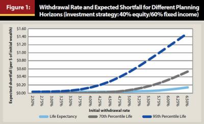
The results in Figure 1 were calculated using Monte Carlo simulation following the method described in the previous section. Expected shortfall was scaled by the initial wealth, so the vertical axis was labeled “expected shortfall per $ of initial wealth.” To get the absolute amount of expected shortfall for this example, readers can simply multiply the per-dollar amount by $1,000,000. Keep in mind that expected shortfall is interpreted as the expected value of the desired retirement spending the retiree will fail to receive. Figure 1 provides a comparison of the risk that would be assessed under different planning horizons or assumed death ages.
The first thing to note in Figure 1 is the very different picture of sustainability risk one gets depending on the planning horizon choice. Consider the base case of an initial withdrawal rate of 5 percent, or $50,000, in the first year. If the planning horizon coincides with the life expectancy, the retiree has a risk of less than $0.01 of shortfall per dollar of initial wealth, or $10,000 for an initial wealth of $1,000,000. If the planning horizon is chosen to be the 70th percentile lifespan from the mortality table, expected shortfall is more than $80,000. At the 95th percentile lifespan, expected shortfall balloons to nearly $510,000. Which risk value is correct? It is not clear.
Another way of thinking about this is in terms of a risk budget. Suppose the retiree does not want to exceed an expected shortfall of $80,000.7 He can then choose an initial spending amount of up to $50,000 if the planning horizon is set at 25 years. However, if the horizon is set at the more conservative 34 years, he must lower his initial spending to less than $40,000 to stay within his allowable risk range. This is a 20 percent reduction in his standard of living. Which risk measure should he use? Either horizon choice could be reasonably justified as “prudent,” but each leads to very different spending decisions.
From this example, it is possible to see that different choices for the length of the planning horizon lead the retiree to very different impressions of where he stands in terms of retirement security and standard of living. Without knowing which one gives the correct measure of risk, the planning advice becomes arbitrary.
The problem of not knowing the correct planning horizon also can lead to the wrong asset allocation advice. So far in the base case example, it was assumed that the retiree had an investment strategy of 40 percent equity and 60 percent fixed income. Now suppose the retiree seeks an investment strategy that minimizes expected shortfall for the base case spending strategy of an initial withdrawal rate of 5 percent with a 2 percent annual cost of living adjustment.
Figure 2 shows how expected shortfall varies with the allocation to equity8 for horizons set at the investor’s life expectancy, the 70th percentile lifespan, and the 95th percentile lifespan. If the horizon is set at the life expectancy, the lowest risk strategy is 100 percent fixed income, although any allocation up to 60 percent equity provides very low expected shortfall. With the horizon set at the life expectancy, expected shortfall is insensitive to the choice of asset allocation over a wide range of values. However, if the horizon is set at the 70th percentile lifespan, the minimum risk strategy is a 20 percent allocation to equity and 80 percent to fixed income. Moving the horizon to the 95th percentile lifespan leads to a higher equity allocation of 60 percent to minimize expected shortfall. More equity is required for longer horizons to up the return and provide better odds of meeting the spending plan.
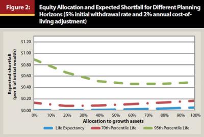
Similar to the spending decision, the planning horizon choice leads to different investment strategies. Which investment strategy should be chosen? It’s unclear without knowing which planning horizon gives the correct assessment of sustainability risk.
Combined, the spending and investment strategy results of this example demonstrate the conundrum of selecting a horizon. Key decisions depend on the assessed risk. The assessed risk depends on the planning horizon choice. There is really no clear guideline on which horizon to choose.
Shorter horizons lead to higher withdrawal rates for the same level of sustainability risk and also lower equity allocations. Such a combination could be disastrous if the retiree outlives the horizon, which is something that could happen with a relatively high probability.
Longer horizons provide a more conservative estimate of the length of time that wealth must last, but sustainability risk likely will be overstated. Consequently, the use of very long horizons may promote low spending and investment strategies with high allocations to equity. Given the potential arbitrary advice that can follow from the wrong risk assessment, the following discussion shows how to find the correct value for expected shortfall.
The Mortality-Adjusting Approach
Sustainability risk depends on two uncertain outcomes: how long one lives and investment returns. Choosing a fixed planning horizon ignores the uncertainty in lifespan, causing the assessed risk measure to deviate from its actual value. Hence, the way to address these incorrect assessments of risk is to explicitly incorporate lifespan uncertainty into the estimate.
The intuition behind the approach is simple. The essential problem with choosing a deterministic planning horizon is that the assessed risk does not pertain to the risk the retiree really cares about; namely, running out of money before running out of life. If an investor is told that he has a 50 percent chance of running out of money by age 100 and his expected shortfall is many times his annual retirement spending, he very well may reduce his spending, even though the information in a mortality table might show he has only a very small chance of living to such an advanced age.
In the approach presented here, the planning horizon is first set so that the investor has a zero chance of outliving it. In the RP 2000 mortality tables produced by the Society of Actuaries that were used here, the maximum assumed age to which a person lives is 116 years. This means that the planning horizon length will change depending on the investor’s age. For example, if the investor is 70 years old, a 46-year planning horizon was used.
Next, for a path of portfolio returns and corresponding spending shortfalls, shortfalls were adjusted by the probability a retiree is alive to experience the failure in sustainability. To illustrate this approach, consider a scenario in which the retiree desires to spend a flat $50,000 per year for his entire life, but runs out of money at age 95 (see Figure 3). With no mortality adjustment, a planner would calculate the shortfall of this scenario as the sum the $50,000 annual payments that are not received between age 95 and 116, arriving at a shortfall of $1,050,000 (21 x $50,000). However, financial planners also need to recognize that these shortfalls will only occur if the investor is alive to experience them.
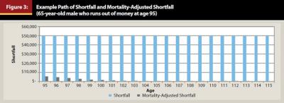
In summing the shortfalls, it is important to multiply each shortfall by the chance of the retiree living to experience the event. For example, the chance of a 65-year-old male living to age 96 and experiencing a shortfall at age 95 is only 11 percent (calculated from the RP 2000 mortality tables). Therefore, the $50,000 increment to shortfall is scaled in this year by 0.11, giving an increment to expected shortfall of $5,500. Similar calculations are estimated for each of the ages out to age 116. Upon summing the mortality-adjusted shortfalls for each period, the expected shortfall is $23,320. This is far less than the non-mortality adjusted shortfall of $1,050,000.
To calculate the expected shortfall across all potential investment outcomes, thereby also accounting for investment uncertainty, Monte Carlo simulations were estimated across investment scenarios. The average of mortality-adjusted shortfall was then taken. This gives an expected shortfall where both investment returns and lifespan are treated as random (alternatively, one can simulate mortality rather than calculating the expectation using probabilities).
This method of mortality-adjusting shortfall takes full account of the fact that there is a chance that the retiree could live to a very old age, but also recognizes that the probability of this happening is small. By using this approach, an adviser will achieve a better estimate of the risk of a client running out of money while still being alive. There is no planning horizon choice that needs to be made in this approach; each possible death age is considered according to its probability.
Mortality-Adjusting Approach Versus Deterministic Planning Horizon Approach
Using the previous example, the risk assessments of the planning horizon choices to mortality-adjusted risk assessments were compared. Figure 4 reproduces Figure 1 for the 65-year-old male investing in a 40 percent equity and 60 percent fixed income portfolio, with the addition of a curve that shows the assessed risk for various withdrawal rates for the mortality-adjusted measure of expected shortfall.
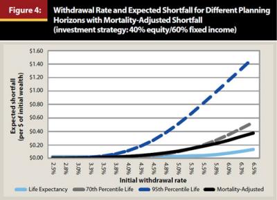
Using the “mortality adjusted” curve in Figure 4, the adviser can help the retiree choose a withdrawal rate based on the expected shortfall risk measure that measures risk as running out of money while still alive. The risk shown by the other curves measures the risk of running out of money at different ages. These deterministic planning horizons represent risk assessments that are based on an adviser’s assessment of lifespan rather than the lifespan estimates of the Society of Actuaries. Figure 5 reproduces Figure 2 with the addition of a curve showing the mortality-adjusted shortfall for different fixed-mix asset allocations.
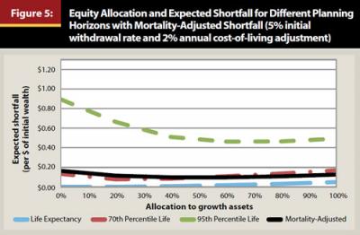
As with the choice of the withdrawal rate, the use of the mortality-adjusting methodology removes the ambiguity in choosing the best investment strategy. Figure 5 also provides an interesting way to compare the influence of the planning horizon choice on the asset allocation decision. This information is captured in Table 1, which shows the fixed allocation that provides the lowest sustainability risk for each planning horizon and the mortality-adjusting methodology.
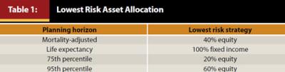
The fixed-mix strategy that minimizes sustainability risk, accounting for mortality, is 40 percent equity and 60 percent fixed income. It is possible that a retiree might choose very different asset allocation strategies depending on the planning horizon. Alternatives range from 0 percent equity to 60 percent equity, if the goal is to minimize shortfall.
Interpreting the mortality-adjusted measure of expected shortfall as the actual sustainability risk for a retiree concerned about running out of money while still alive, as shown in Figures 4 and 5, illustrates the error created by using different deterministic horizons to support the choices of withdrawal rate and investment strategy. The life expectancy and the 95th percentile life calculations provide poor approximations of the true sustainability risk shown by the “mortality-adjusted” curves, but the 70th percentile lifespan horizon appears to provide a reasonable approximation. However, it does lead to a different investment strategy choice.
It is important to keep in mind that the reasonable approximations provided by the 70th percentile deterministic horizon is not a general result. It holds for the hypothetical retiree in the example, but it might not hold based on other assumptions of age, gender, and asset returns.
Additionally, while it may be possible that a deterministic planning horizon could be used to approximate mortality-adjusted risk, this approach is not recommended. It would be necessary to calculate the mortality-adjusted risk measure for each set of investment return assumptions, withdrawal rate, age, gender, and other factors to find the deterministic horizon that provides the best approximation. Therefore, calculating the mortality-adjusted approach is unavoidable. Once this calculation has been made with a spending plan determined, there is no need to find the deterministic age that reproduces the same risk.
Conclusions and Implications
Representing sustainability risk accurately is important because retirees and their advisers base spending decisions and investment decisions on this risk. This paper shows that measuring sustainability risk relative to different deterministic planning horizons causes significantly different assessments of sustainability risk. Without the knowledge of the actual sustainability risk value, planners will not know how large of an error there is in their estimate of a spending plan’s sustainability risk.
An approach to measure sustainability risk that expresses the true risk faced by a retiree was described: the joint occurrence of running out of money while still being alive. In comparing spending and investment decisions derived from deterministic horizons to those derived from the mortality-adjusting approach, significant differences were noted.
Typically, financial planners err on the side of choosing a conservative (long) planning horizon to protect against their clients outliving their assets. One might argue that conservatism in retirement planning is prudent. This paper posits an important difference between conservatism based on an overstatement of sustainability risk and a conservative spending or investment decision based on an accurate measure of sustainability risk. An adviser’s clients should base decisions on an accurate assessment of risk, not one that has a conservative buffer built into it. Otherwise, clients cannot make efficient tradeoffs between sustainability risk and spending decisions. Further, inefficient asset allocations will be chosen.
Computing mortality-adjusted risk assessments can be done either formulaically as shown in this paper, or mortality events can be simulated similarly to investment returns. Practically speaking, either of these approaches needs to be built into a planning tool rather than used to determine a rule for setting the deterministic planning horizon that can be used in an existing tool. The deterministic horizon that best approximates the mortality-adjusted approach depends on the inputs of a spending plan, including age, gender, marital status, spending amounts, cost of living assumptions, and other variables. In other words, one would have to build a planning tool based on mortality-adjusting to determine the deterministic planning horizon that best approximates the risk of the mortality-adjusted approach. However, once the tool that produces the actual sustainability risk is in place, there is no reason to find the deterministic horizon that approximates the mortality-adjusted risk unless one is curious.
Planning software and tool providers can help advisers and their clients make more efficient spending and investment decisions by incorporating lifespan uncertainty into their planning tools. The potential errors in sustainability risk assessment caused by using an arbitrarily chosen deterministic planning horizon, and the inefficiency that these errors introduce into retirement decision making, are too large to ignore.
Endnotes
- In a research report by the Society of Actuaries (Turner and Witte 2009), 12 retirement planning software tools were reviewed, in which none explicitly include lifespan uncertainty.
- Much of the published work on choosing an appropriate planning horizon concerns sustainable withdrawal rates. The classic study was authored by Bengen (1994). See also, Kitces (2008), Pfau (2011), Blanchett (2007), Frank et al. (2011), and Fullmer (2009a). These researchers used deterministic planning horizons. More recently, several authors have investigated directly including lifespan uncertainty into the planning problem. See Milevsky and Huang (2011), Finke et al. (2012), and Blanchett et al (2012).
- Many financial planners use the probability of plan failure to measure risk. The general argument of not using a single deterministic planning horizon applies to the assessment of probability of failure, too. The expected shortfall is used because, as a risk measure, it reflects both the chance of failure and the magnitude of failure.
- See Fullmer (2009b) for a complete description of measuring shortfall risk.
- The appendix shows the return assumptions associated with equity and fixed income used for all analyses in this paper.
- Although this discussion focuses on the base case, Figures 1 and 2 contain information for the interested reader to consider a variety of cases with different withdrawal rates and asset allocations.
- This risk budget statement could be stated analogously as, “I don’t want the probability of failure for my spending plan to be more than 80 percent.”
- Simulated allocations of 0 percent/100 percent; 20/80; 40/60; 60/40; 80/20 and 100/0 equity to fixed income were used to draw these curves.
References
Bengen, William P. 1994. “Determining Withdrawal Rates Using Historical Data.” Journal of Financial Planning 7 (4): 171–180 (October).
Blanchett, David M. 2007. “Dynamic Allocation Strategies for Distribution Portfolios: Determining the Optimal Distribution Glide Path.” Journal of Financial Planning 20 (12): 68–81.
Blanchett, David M., Maciej Kowara, and Peng Chen. 2012. “Optimal Withdrawal Strategy for Retirement Portfolios.” The Retirement Management Journal 2 (3): 7–20.
Fan, Yuan-An, and Grant W. Gardner. 2012. “Russell’s Adaptive Investing Methodology.” Russell Investments Research White Paper. www.russell.com/AU/_pdfs/capital-markets-reserach/forum/R_NEWS_Forum_Adapt_V1F_WEB_1108.pdf.
Fan, Yuan-An, Steve Murray, and Sam D. Pittman. 2013. “Optimizing Retirement Income: An Adaptive Approach Based on Assets and Liabilities.” The Journal of Retirement 1 (1): 124–135.
Finke, Michael, Wade D. Pfau, and Duncan Williams. 2012. “Spending Flexibility and Safe Withdrawal Rates.” Journal of Financial Planning 25 (3): 44–51.
Frank, Larry, John Mitchell, and David Blanchett. 2011. “Probability-of-Failure-Based Decision Rules to Manage Sequence Risk in Retirement.” Journal of Financial Planning 24 (11): 44–53.
Fullmer, Richard K. 2009a. “A Framework for Portfolio Decumulation.” Journal of Investment Consulting 10 (1): 63–71.
Fullmer, Richard K. 2009b. “Mismeasurement of Risk in Financial Planning.” Russell Investments Research White Paper. www.plansponsor.com/uploadfiles/Russell.pdf.
Guyton, Jonathan T. 2004. “Decision Rules and Portfolio Management for Retirees: Is the ‘Safe’ Initial Withdrawal Rate Too Safe?” Journal of Financial Planning 17 (10): 54–62.
Guyton, Jonathan T., and William J. Klinger. 2006. “Decision Rules and Maximum Initial Withdrawal Rates.” Journal of Financial Planning 19 (3): 50–58.
Kitces, Michael E. 2008 (May). “Resolving the Paradox—Is the Safe Withdrawal Rate Sometimes Too Safe?” The Kitces Report. www.kitces.com/may-2008-issue-of-the-kitces-report/.
Milevsky, Moshe A., and Huaxiong Huang. 2011. “Spending Retirement on Planet Vulcan: The Impact of Longevity Risk Aversion on Optimal Withdrawal Rates.” Financial Analysts Journal 67 (2):45–58.
Pfau, Wade D. 2011. “Safe Savings Rates: A New Approach to Retirement Planning over the Life Cycle.” Journal of Financial Planning 24 (5): 42–50.
Turner, John A., and Hazel A. Witte. 2009. “Retirement Planning Software and Post-Retirement Risks: Highlights Report.” Society of Actuaries White Paper.
Citation
Gardner, Grant, and Sam Pittman. “Measuring the Risk of Running Out of Money in Retirement.” Journal of Financial Planning 26 (12): 38–44.