Increasing the Sustainable Withdrawal Rate Using the Standby Reverse Mortgage

​Journal of Financial Planning: December 2013

 

 

Executive Summary

• This study investigates maximum real sustainable withdrawal rates (SWRs) for retirement plans that incorporate the use of standby reverse mortgages (SRMs). The SWR is defined as the maximum real withdrawal rate with a minimum 90 percent plan survival rate for a 30-year retirement horizon.
• The SRM evaluated in this study is a Home Equity Conversion Mortgage (HECM) reverse mortgage line of credit that is established at the beginning of retirement and is used for retirement income during bear markets. Outstanding loan balances are repaid from the Investment Portfolio (IP) in bull markets.
• Monte Carlo simulations were used to estimate the success of the SRM strategy at various real withdrawal rates for a client who has a $500,000 investment nest egg and $250,000/$500,000 in home equity at the beginning of retirement. The $500,000 nest egg is split into a 60 percent stocks and 40 percent bonds IP and a six-month cash reserve.
• Retirees who begin retirement in a low interest rate environment (2.3 percent yield on 10-year U.S. Treasury bond) with competitive lending terms and significant home equity relative to the IP stand to benefit the most from an SRM strategy. Interest rates and the size of the initial line of credit relative to the IP are the two factors that are shown to have a significant impact on the SWR for the SRM distribution strategy.
• Results pertaining to the low interest rate and current lending environment indicate that a 5.0 percent SWR is attainable for the SRM strategy when home equity is at least 50 percent of the IP at retirement. The SWR for the SRM strategy is estimated to be as high as 6.75 percent for retirees in the low interest rate environment where home equity is equal to the IP at the beginning of retirement.

Shaun Pfeiffer, Ph.D., is an associate professor of finance and personal financial planning at the Edinboro University of Pennsylvania. Email HERE.

John Salter, Ph.D., CFP^®, AIFA^®, is an associate professor of personal financial planning at Texas Tech University and wealth manager at Evensky & Katz Wealth Management in Coral Gables, Florida and Lubbock, Texas. Email HERE.

Harold Evensky, CFP^®, AIF^®, is a research professor of personal financial planning at Texas Tech University and the president of Evensky & Katz Wealth Management in Coral Gables, Florida and Lubbock, Texas. Email HERE.

Acknowledgement: The authors thank Liberty Home Equity Solutions Inc. for sponsoring and providing necessary loan data for this research study.

Research published in the Journal of Financial Planning has estimated that retirees can expect to safely withdraw roughly 4 percent of their initial portfolio value, adjusted for inflation, each year in retirement (Bengen 1994). However, recent research has questioned whether the 4 percent rule is safe for retirees who are projected to face lower returns than those experienced by previous generations (Finke, Pfau, and Blanchett 2013; Pfau 2012).

The concern for provision of adequate real retirement income has led to another recent study that found the use of a Home Equity Conversion Mortgage (HECM) Saver reverse mortgage line of credit, referred to as the standby reverse mortgage (SRM) strategy, significantly reduced shortfall risk for retirees facing lower future returns when compared to strategies that do not use the HECM Saver (Salter, Pfeiffer, and Evensky 2012). However, these authors did not estimate the maximum real sustainable withdrawal rate (SWR) for the SRM strategy. This study adds to the literature by estimating the SWR for an SRM strategy based on the new HECM reverse mortgage over the course of 30 years for a 10 percent maximum acceptable failure rate, for a retiree who uses the SRM strategy in a retirement where returns are projected to be lower than seen historically. The new HECM product, explained below, replaced the HECM Saver and Standard in October 2013.

Background Review

Bengen (1994) established the 4 percent rule when he investigated distributions from a stock and bond portfolio using historical data. Subsequent research has examined the SWR under various distribution assumptions and has estimated the SWR to have an approximate range of 2.5 percent to 6 percent. This range is attributable to a variety of assumptions, such as partial annuitization, asset allocation, longevity, expected returns and volatility, tax efficiency of the strategy, and willingness to adjust withdrawals after poor market performance (Salter and Evensky 2008).

The SWR estimates that cluster near 6 percent have been primarily associated with distribution strategies that include partial annuitization of retirement savings (Ameriks, Veres, and Warshawsky 2001) or dynamic rules for withdrawal rates in a given year (Guyton 2004). However, research has shown that private annuities are largely ignored by retirees as evidenced by the finding that they account for less than 2 percent of total wealth for retirees (Johnson, Burman, and Kobes 2004). In addition, studies have documented that significant changes in retirement income are associated with diminished success of the adviser (King 2012) and diminished client satisfaction due to not achieving a goal (Calvo, Haverstick, and Sass 2009). In other words, dynamic withdrawal strategies that could potentially require significant changes in retirement income may be inappropriate for many retirees.

Retirees who resist annuitization and dynamic, or variable, withdrawal strategies are unlikely to be impressed by the SWR estimates in a low return environment as suggested by notable investment professionals (Arnott and Bernstein 2002; Cornell 2010). For example, Pfau (2012) examined the SWR under less optimistic capital market expectations than seen historically. Pfau found that a 1.3 percent reduction in real average annual stock return projections, from the historical 8.7 percent to 7.4 percent, is sufficient to decrease the SWR below 4 percent. Finke, Pfau, and Blanchett (2013) went a step further and showed that a combination of negative annual real bond returns and a 6 percent annual equity premium assumption can lead to a SWR as low as 2.5 percent.

Some retirees will be in a position to tolerate such a low SWR due to other resources. However, recent studies have suggested that the typical retiree has limited resources. For example, one study reported that less than 20 percent of current retirees have a defined benefit pension plan (Butrica, Smith, Toder, and Iams 2009), and that the median value of IRAs and 401(k)s stands near $120,000, while median financial assets outside of retirement savings are approximately $30,000 (Munnell and Rutledge 2013). In short, the typical retiree is likely to find that a low SWR has a meaningful negative impact on his or her standard of living in retirement.

Given market conditions in the current retirement landscape, two researchers have stated that “Housing equity is likely to become an increasingly important source of support as retirement needs rise and the retirement income system contracts” (Munnell and Rutledge 2013, p. 10). Fortunately, home equity is a significant source of wealth for the typical retiree. Prior research has found home equity to be between 45 percent and 75 percent of net worth for the median household approaching retirement (Fisher, Johnson, Marchand, Smeeding, and Torrey 2007; Lusardi and Mitchell 2007). In addition, a fairly recent report indicated that the median home value for households over the age of 65 to be $150,000 nationwide and as high as $230,000 in the western region of the United States (Szymanoski and Johnson 2011). Despite the documented rise of mortgage debt among older households (Smith, Finke, and Huston 2012) studies have shown that a significant number of retirees have little to no mortgage debt (Timmons and Naujokaite 2011).

Reverse mortgages represent one option retirees can use to tap home equity in retirement. However, retirees historically have been resistant to the idea of reverse mortgages despite the significance of home equity as a portion of total wealth. This resistance in the past has been attributed primarily to high upfront fees of up to 7 percent, with origination costs, of the home value (Davidoff and Welke 2004). Fortunately, a less costly reverse mortgage, the HECM, became available to seniors in October 2013.¹ The upfront costs for the HECM are lower than the upfront costs of the Standard option by 1.5 percent, or more, depending on the lending environment (Salter, Pfeiffer, and Evensky 2012). Upfront costs include the typical mortgage costs of title insurance, appraisals, and attorney fees, plus a FHA mortgage insurance premium of 2 percent for the Standard HECM or 0.50 percent for a HECM, and any applicable origination costs that vary across lenders.

In the past, the media has focused on the costs of reverse mortgages rather than potential benefits (Lewin 2001). Recently, research has focused on both the cost and potential benefits of reverse mortgages in retirement planning. For example, Salter, Pfeiffer, and Evensky (2012), using the 30-year mark in retirement for a 5 percent real withdrawal rate, estimated shortfall risk for the SRM distribution strategy to be 50 percent lower than the shortfall risk for a distribution strategy that did not use a HECM Saver reverse mortgage. In addition, these authors found that the SRM strategy incurred no meaningful reduction in wealth at the 30-year horizon when compared to the wealth of the strategy that did not use the HECM Saver.

Similarly, another study examined the more costly HECM Standard reverse mortgage in retirement and found significant reductions in shortfall risk at the 30-year mark when compared to distribution strategies that either failed to incorporate the use of the HECM Standard or used it as a last resort (Sacks and Sacks 2012). The findings from these studies suggest that a thoughtful distribution strategy that incorporates reverse mortgages can lead to meaningful reductions in shortfall risk despite the costs that are incurred by using the products.

Investigating the Standby Reverse Mortgage Strategy

This study is most similar to the small strand of empirical research that uses reverse mortgages in retirement planning (Sacks and Sacks 2012; Salter, Pfeiffer, and Evensky 2012). The findings from this study add to the existing literature by estimating the SWR for an SRM distribution strategy that uses the new HECM reverse mortgage. The robustness of the SRM distribution strategy is tested under an environment of lower capital market expectations where different interest rate environments and home equity values are taken into account. The variation in interest rate environments is important due to the concern for increasing rates in the future, whereas different home equity assessments illustrate the greater impact of an SRM strategy when home equity increases relative to the portfolio value.

The SRM strategy is best described as a three-bucket strategy. The first bucket is the IP, which has been simplified in this study to a 60 percent/40 percent mix of stocks and bonds. The equity assumptions are based on a diversified large cap core domestic position, whereas the bond assumptions are based on a diversified intermediate-term domestic taxable bond position.

The second bucket, called the Standby Bucket, is the HECM line of credit, which may be used and paid back without taxation at the discretion of the retiree. The IP and Standby Bucket are used to refill the third bucket, the Cash Bucket, which is six months of forward-looking income needs in the form of cash reserves, which provide income to the retiree.

Determination of use and payback of the Standby Bucket is based on a glide path that is derived from a capital needs analysis. The portfolio value line is the theoretical glide path a financial planner would expect his or her client portfolios to follow to meet goals. Put differently, the glide path represents the value of the portfolio across time that would allow the client to fully fund the real withdrawal rate for each year in a 30-year retirement horizon. In practice, the capital needs analyses are updated over time to account for changes in capital market assumptions and/or client needs. Therefore, the glide path and triggers for use and payback of the Standby Bucket would adjust according to the updated glide path. However, in this study the glide path was fixed from the onset of simulations.

After extensive analysis, it was determined that 80 percent of the glide path is the optimal level to determine use and payback of the Standby Bucket (Salter, Pfeiffer, and Evensky 2012). This assessment was based on SRM survival rates and use of the line of credit. Therefore, the use of the glide path for a client who has $500,000 today, using the projected returns, would be expected to have $508,660 at the end of the year after a 5 percent distribution at the beginning of the year. One year later, 80 percent of the post distribution glide path value, or $406,948, would be compared to the IP to determine whether the IP or Standby Bucket should refill cash reserves, if applicable.² Using 100 percent or 90 percent resulted in over use of the line of credit, which led to poorer results when compared to the 80 percent mark.

At the beginning of each quarter, income needs are met by the Cash Bucket. The Cash Bucket, once depleted, is refilled at the end of the quarter. It is important to note that the Cash Bucket is not refilled every quarter; however, it must be refilled at least two times each year. Similarly, the outstanding loan balance is paid down at the end of the quarter if the IP exceeds the glide path. The SRM strategy proceeds on a quarterly basis as follows:

When the IP is equivalent to or exceeds the glide path:

• IP pays off any loan balance then refills Cash Bucket if needed.
• IP refills the Cash Bucket when rebalancing or the Cash Bucket is empty. In practice, refills also would occur if any investment changes were made due to a change in client goals and/or capital market expectations. (Note: A minimum $3,000 loan balance is needed for loan payoff to occur when the Cash Bucket is not refilled due to concern for transaction costs. In other words, this minimum loan balance is set so a transaction cost is not incurred to pay off relatively small loan balances.)

When the IP is less than the glide path:

• Once the Cash Bucket is sufficient, it is only necessary to rebalance and/or make investment changes and use the Standby Bucket (that is, borrow from line of credit, to the extent available, to refill the Cash Bucket).

Methodology

This analysis was based on 1,000 Monte Carlo simulations to estimate the SWR for the SRM strategy. Each of the simulations represents a hypothetical economic environment during retirement with different IP return patterns and interest rates. Each simulation incorporated up to 156 quarters, or 39 years, worth of information on investment returns, interest rates, volatility, and transaction costs. Transaction costs were held constant at $30 per transaction. Interest rates and investment returns were stochastic. Income needs were met by using the cash reserve account. The cash reserve account was refilled by either the HECM line of credit or the IP based on the SRM strategy.

The following discussion outlines the HECM and the capital market assumptions underlying this study.

HECM. The HECM Saver was introduced in October 2010 as a less costly reverse mortgage option to retirees who are at or above the age of 62 and want to access home equity in a tax-free manner (Kitces 2011). The HECM, introduced in October 2013, replaces the HECM Saver. The SRM strategy in this study uses the line of credit option available from the HECM; however, annuity payments, and a combination of payments and a line of credit are also available. The costs of this product can be bifurcated into upfront costs and ongoing costs associated with the establishment and use of the HECM. These costs vary across lenders. The benefit of this product is a noncancellable line of credit that may be used at the discretion of the borrower free of taxes.

The upfront costs include closing costs, origination fees, and a Mortgage Insurance Premium (MIP). A report from AARP documented the typical range for closing costs to be between $2,000 and $3,000 (AARP 2011). The origination fee is capped at 2 percent of home value up to the first $200,000 in value and 1 percent above that with a maximum of $6,000 (U.S. Department of Housing and Urban Development 2011). The MIP for the HECM is currently 0.50 percent, or $1,250, for a $250,000 home at establishment date. For this study, it was assumed that the summation of origination fees and closing costs is 3.50 percent of the home value on establishment date. This is attainable in the current lending environment; however, this figure may be lower than that quoted by some lenders.³

Ongoing costs include interest costs when and if the funds are borrowed. The ongoing interest consists of a variable interest rate that changes monthly, the lender’s margin set at date of origination, and an annual 1.25 percent MIP charged by the Federal Housing Administration (FHA).

The variable interest rate is indexed to the one-month LIBOR rate, which as of November 2013 was 0.20 percent. This variable rate is adjusted monthly. This study assumed a lender’s margin of 3.0 percent; however, this will vary across lenders. In today’s environment, a borrower would initially face a total annual effective interest rate of 4.50 percent. Roughly 1/12 th of this rate accrues to any outstanding loan balance on a monthly basis. Using history as a guide, this study accounts for the variability in LIBOR rates by simulating a 5.0 percent average rate with a range between 0.20 percent and 12 percent.

The benefit of this line of credit product is initially determined by the Principal Limit Factor (PLF). The PLF is the percent of home equity that is available in the form of a line of credit at the time of origination. The age of the youngest borrower and the expected interest rate at loan origination date are the two factors that determine the PLF. The PLF tables for various interest rates and ages of the youngest borrower are made available by the U.S. Department of Housing and Urban Development.⁴ The expected interest rate is the summation of the 10-year LIBOR swap rate and the lender’s margin. The PLF increases with age and decreases as the expected interest rate rises. It is important to note that the 10-year LIBOR swap rate has a direct impact on the amount of home equity that can be accessed through a reverse mortgage. However, the one-month LIBOR rate represents a portion of the effective interest rate that accrues on an outstanding loan and does not directly impact the PLF.

This study assumed that the line of credit is established at age 62 with a 3.0 percent lender margin. A 10-year LIBOR swap rate of 2.4 percent, as seen in the summer of 2013, leads to an expected interest rate of 5.4 percent and a PLF of 47.9 percent in a low interest rate environment. Based on this information, a 62-year-old borrower with $250,000 in home equity would have access to a $119,750 line of credit before upfront costs are paid.

This study reports results based on a low, moderate, and a high interest rate environment where the corresponding PLFs are 47.9 percent, 34.3 percent, and 18.5 percent, respectively. For a 3.0 percent lender’s margin, these PLFs correspond with a 2.4 percent, 4.0 percent, and 7.0 percent 10-year LIBOR swap rate, respectively. Federal Reserve data⁵ on the 10-year LIBOR swap rate begins in July 2000. Since then, this rate has been, on average, roughly 40 basis points higher than the yield on the 10-year U.S. Treasury bond.

Capital market assumptions. This study assumed an average annual nominal pre-tax return of 8.75 percent for stocks, 4.75 percent for bonds, and 3.50 percent for cash with inflation projected at 3.0 percent. Annualized standard deviations were 21.0 percent, 6.5 percent, and 2.0 percent for stocks, bonds, and cash, respectively. The correlation of stocks to bonds was modeled at 30 percent, and inflation was assumed to be constant at 3.0 percent each year. These return and volatility assumptions are in line with the latest forward looking projections provided by the MoneyGuidePro software. Transaction costs were set at $30 per trade and distributions were assumed to be gross of taxes. The IP was rebalanced at 5 percent absolute deviation from the initial asset allocation.⁶

The one-month LIBOR rate was modeled with a projection of 5.0 percent, with a range of 0.2 percent to 12.0 percent. The lender’s margin and annual ongoing MIP were held constant at 3.0 percent and 1.25 percent. Upfront costs were assumed to be 3.5 percent of the home value on origination date. This study examines starting home values of $250,000 and $500,000 in relation to a constant beginning portfolio value of $500,000. The analysis was used to examine a 47.9 percent, 34.3 percent, and 18.5 percent PLF to account for low, moderate, and high interest rate environments, respectively.

Results

SRM survival rates are shown for the 30-year mark in retirement. This paper examines the survival rates for real withdrawal levels between 3.25 percent and 7.00 percent, in increments of 0.25 percent. All results are based on 1,000 simulations for each real withdrawal rate. In turn, the SWR represents the maximum real withdrawal rate that supports a minimum acceptable survival rate of 90 percent, or a maximum acceptable failure rate of 10 percent. Two strategies are shown for each real withdrawal rate where both strategies begin with a $500,000 nest egg at the beginning of retirement in all scenarios. The SRM strategy is based on a client who establishes a SRM at age 62 and has either $250,000 or $500,000 in home equity at the beginning of retirement. The No SRM strategy is based on a client who does not establish an SRM and simply relies on the retirement savings throughout retirement. The impact of different interest rate environments and different home equity levels can be seen in the figures and tables. Both strategies assume the use of a six-month cash flow reserve.

Figure 1 shows results in 0.50 percent increments and pertains to the case scenario of a client with a $250,000 home value who begins retirement in a low interest rate environment. Based on the 90 percent minimum acceptable survival rate, all of the SRM withdrawal rates (except for 5.25 percent) are estimated in the acceptable range. However, none of the withdrawal rates for the No SRM strategy in Figure 1 are estimated to be acceptable. More specifically, the SRM strategy is estimated to support an SWR of roughly 5.0 percent based on the 90 percent survival rate at year 30, whereas the SWR for the No SRM strategy is slightly less than 3.25 percent. Said differently, the SRM SWR is estimated to be roughly 1.75 percentage points higher than the No SRM SWR.⁷

 

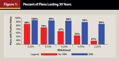
The SWR for the No SRM strategy of 3.25 percent sheds light on the capital market assumptions in relation to the smaller SWR of 2.50 percent reported by Finke, Pfau, and Blanchett (2013). That is, the capital market assumptions are not as optimistic as historical data would suggest; however, when compared to the previous study, the assumptions appear to be slightly more generous. In unreported results, the SRM SWR was estimated to be 4.25 percent for a $100,000 home value and a $500,000 nest egg. The diminished appeal of the SRM strategy for a $100,000 home value is due to higher relative upfront fees that were assumed to be 5.0 percent of the home value.

Table 1 illustrates the survival rates and median wealth for the SRM and No SRM strategies at the 30-year mark in retirement for home equity levels of $250,000 and $500,000 in a low interest rate environment. The low interest rate environment corresponds with a 47.9 percent PLF. The PLF in Panel A leads to a $119,750 initial line of credit, whereas the PLF in Panel B leads to a $239,500 initial line of credit.

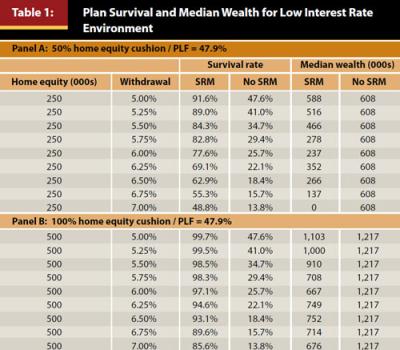
When home equity and portfolio values are $250,000 / $500,000, as seen in Panel A of the table, then the home equity cushion is equal to 50 percent. The results span 5.0 percent to 7.0 percent real withdrawal rates in 0.25 percent increments. The SRM SWR in Panel A of approximately 5.0 percent, as evidenced by the above 90 percent survival rate, is roughly 1.75 percent lower than the SRM SWR of 6.75 percent in Panel B. This is due to the difference in home equity assumptions. Note that the failure rate (1 – survival rate) for the SRM strategy in both panels shows the percent of simulations that have exhausted the IP, cash reserves, and the line of credit.

The conclusions from Table 1 are twofold. First, an SRM strategy is estimated to boost the SWR by as much as 3.50 percent when compared to the SWR of 3.25 percent for a No SRM strategy. In addition, a higher home equity cushion increases the SWR advantage of the SRM relative to the No SRM strategy as evidenced by the higher survival rates in Panel B when compared to the survival rates for the same withdrawal rates in Panel A. Finally, median wealth for the SRM strategy at the 5.0 percent withdrawal rate in Panel A is roughly 3.30 percent or $20,000 lower than the median wealth for the No SRM strategy. However, this estimated reduction in median wealth for the SRM strategy at the 5.0 percent withdrawal rate is associated with an estimated survival rate increase of roughly 44 percentage points relative to the No SRM strategy.

The same comparisons in Panel B at the 6.75 percent withdrawal rate show the SRM median wealth is estimated to be $503,000 or 41 percent lower than the median wealth of the No SRM strategy; however, this reduction in wealth leads to an estimated 74 percentage point increase in survival rate.

Table 2 sheds light on the SRM SWR in moderate and high interest rate environments where the 10-year LIBOR swap rates are 4.0 percent and 7.0 percent on loan origination dates at the beginning of retirement. Panel A shows the results for a high interest rate environment where the line of credit for the SRM strategy is 18.5 percent of the home value at the beginning of retirement. The results indicate that a high interest rate environment takes a toll on the SRM SWR. Specifically, the SRM SWR is estimated to be 4.0 percent in a high interest rate environment where home equity is half the value of retirement savings at the onset of retirement. Said differently, high interest rates, at origination date, diminish the SRM SWR by approximately 1.0 percent when compared to the estimated SRM SWR of 5.0 percent in Panel A of Table 1.

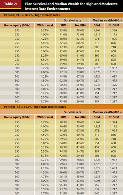
The SRM SWR advantage in Panel A of Table 2 of approximately 0.75 percent, in comparison to the 3.25 percent estimated No SRM SWR in Figure 1, is coupled with a slight reduction in median wealth of roughly 5 percent when compared to the median wealth of the No SRM SWR as seen in the last two columns for the 4.0 percent real withdrawal rate. In sum, Panel A suggests that the establishment of an SRM strategy becomes less attractive in a high interest rate environment and that interest rates at the time of origination should be weighed heavily by the practitioner and/or retiree when deciding whether a HECM SRM should be established.

Panel B of Table 2 shows results for a line of credit and PLF that are 34.3 percent of the home value. The results indicate that a 4.75 percent and 5.75 percent SWR is attainable for an SRM strategy where $250,000 and $500,000 of home equity is used to establish a line of credit in a moderate interest rate environment. These estimates indicate that a meaningful SRM SWR advantage, reported to be as high as 2.5 percent, remains intact in a moderate interest rate environment when compared to the No SRM strategy SWR of approximately 3.25 percent as seen in Figure 1.

Median wealth figures for the 4.75 percent withdrawal rate, or estimated SRM SWR, in the upper half of Panel B is estimated to be $38,000 or 5.3 percent lower than median wealth for the No SRM strategy. However, the median wealth results for the 5.75 percent real withdrawal rate in the lower half of Panel B suggest that the 62 percentage point estimated increase in survival rate for the SRM strategy in relation to the No SRM strategy is coupled with a 47 percent reduction in median wealth.

Figure 2 places all of the findings across interest rate and home equity scenarios into one snapshot. This figure indicates that the SRM SWR is estimated to be as low as 4.0 percent in a high interest rate environment with a 50 percent home equity cushion, and as high as 6.75 percent in a low interest rate environment with a 100 percent home equity cushion. In short, the SRM SWR increases with a home equity cushion and decreases with the interest rate environment at loan origination date.

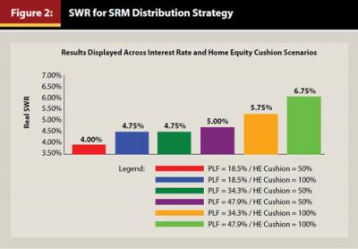
It is important to remember that the PLF values in Figure 2 correspond to each of the panels in the Tables 1 and 2. In other words, the PLF value is equal to the percent of home equity at retirement date that is available in the form of a line of credit.

Conclusion

The primary conclusion of this study is that the implementation of a thoughtful SRM strategy in moderate and low interest rate environments can boost the SWR, relative to a No SRM strategy SWR of approximately 3.25 percent, by roughly 1.50 percent to 3.50 percent.

These results are dependent upon the interest rate environment and home equity cushion at the loan origination date. Stated another way, an SRM SWR is estimated to be between 5.75 percent and 6.75 percent when established by retirees with a 100 percent home equity cushion in moderate and low interest rate environments, respectively.

The results also suggest minimal to modest reductions in median wealth at the 30-year mark for a SRM strategy with a 50 percent home equity cushion at the beginning of retirement when compared to the No SRM strategy. However, the SRM strategy SWR advantage over the No SRM SWR in scenarios where the home equity cushion is 100 percent is accompanied by a more significant reduction in median wealth.

In addition, it is important to note that the SRM SWR advantages over the No SRM strategy diminish significantly as high interest rates are experienced at origination date. The rationale for this finding is that high interest rates lead to much lower lines of credit for borrowers, and ultimately, a higher cost-to-benefit ratio.

Together, these findings suggest that the adage of using a reverse mortgage as a last resort could be a huge mistake in a rising interest rate environment where a retiree waits to set up a line of credit in the future. In addition, the current retirement landscape, due to low interest rates, should incentivize the consideration of reverse mortgages in retirement for many financial planners and their clients.

Endnotes

1. U.S. Department of Housing and Urban Development. 2013. Changes to HECM Program Requirements. http://portal.hud.gov/hudportal/HUDsrc=/program_offices/housing/sfh/hecm/hecmml.
2. This calculation is based on a 7.15 percent expected portfolio return derived from the 8.75 percent and 4.75 percent expected return on stocks and bonds. In addition, a constant 3 percent inflation rate that increases quarterly withdrawals was assumed.
3. Multiple quotes from Liberty Home Equity Solutions and Ibis were reviewed. The range of total upfront costs was between 2.0 percent and 3.5 percent for homes valued between $250,000 and $500,000 at origination date and as high as 5.5 percent for a $100,000 home.
4. See: portal.hud.gov/hudportal/HUDsrc=/program_offices/housing/sfh/hecm/hecmhomelenders.
5. See: www.federalreserve.gov/releases/h15/data.htm.
6. No meaningful difference in unreported results for a 5 percent and 10 percent rebalancing band were detected.
7. The estimated SWR for the No SRM in this strategy was 3.15 percent and was not included in the figure for visual reasons. These results will be provided upon request.

References

AARP. 2011. “Reverse Mortgage Loans: Borrowing Against Your Home.”

Ameriks, John, Robert Veres, and Mark J. Warshawsky. 2001. “Making Retirement Income Last a Lifetime.” Journal of Financial Planning 14 (12): 60–76.

Arnott, Robert D., and Peter L. Bernstein. 2002. “What Risk Premium is “Normal”?” Financial Analysts Journal 58 (2): 64–85.

Bengen, William P. 1994. “Determining Withdrawal Rates Using Historical Data.” Journal of Financial Planning 7 (4): 171–180.

Butrica, Barbara A., Karen E. Smith, Eric Toder, and Howard M. Iams. 2009. “The Disappearing Defined Benefit Pension and Its Potential Impact on the Retirement Incomes of Boomers.” Available online from the Center for Retirement Research at Boston College.

Calvo, Esteban, Kelly Haverstick, and Steven A. Sass. 2009. “Gradual Retirement, Sense of Control, and Retirees’ Happiness.” Research on Aging 31 (1): 112–135.

Cornell, Bradford. 2010. “Economic Growth and Equity Investing.” Financial Analysts Journal 66 (1): 54–64.

Davidoff, Thomas, and Gerd Welke. 2004. “Selection and Moral Hazard in the Reverse Mortgage Market.” Social Science Research Network. papers.ssrn.com/sol3/papers.cfm?abstract_id=608666.

Finke, Michael, Wade D. Pfau, and David M. Blanchett. 2013. “The 4 Percent Rule Is Not Safe in a Low-Yield World.” Journal of Financial Planning 26 (6): 46–55.

Fisher, Jonathan D., David S. Johnson, Joseph T. Marchand, Timothy M. Smeeding, and Barbara B. Torrey. 2007. “No Place Like Home: Older Adults and Their Housing.” Journal of Gerontology 62 (2): S120–S128.

Guyton, Jonathan T. 2004. “Decision Rules and Portfolio Management for Retirees: Is the ‘Safe’ Initial Withdrawal Rate Too Safe?” Journal of Financial Planning 17 (10): 54–62.

Johnson, Richard W., Leonard E. Burman, and Deborah Kobes. 2004. “Annutized Wealth at Older Ages: Evidence from the Health and Retirement Study.” Urban Institute. www.urban.org/url.cfm?ID=411000.

King, Rebecca. 2012. “Finding Success in Retirement Income Planning.” Journal of Financial Planning 25 (12): 38–41.

Kitces, Michael E. 2011. “A Fresh Look at the Reverse Mortgage.” The Kitces Report (October).

Lewin, Fereshteh A. 2001. “The Meaning of Home among Elderly Immigrants: The Directions for Future Research and Theoretical Development.” Housing Studies 16 (3): 353–370.

Lusardi, Annamaria, and Olivia S. Mitchell. 2007. “Baby Boomer Retirement Security: The Roles of Planning, Financial Literacy, and Housing Wealth.” Journal of Monetary Economics 54 (1): 205–224.

Munnell, Alicia H., and Matthew S. Rutledge. 2013. “The Effects of the Great Recession on the Retirement Security of Older Workers.” Center for Retirement Research at Boston College. National Poverty Center Working Paper Series. www.npc.umich.edu/publications/working_papers/.

Pfau, Wade. 2012. “Capital Market Expectations, Asset Allocation, and Safe Withdrawal Rates.” Journal of Financial Planning 25 (1): 36–43.

Sacks, Barry H., and Stephen R. Sacks. 2012. “Reversing the Conventional Wisdom: Using Home Equity to Supplement Retirement Income.” Journal of Financial Planning 25 (2): 43–52.

Salter, John R., and Harold R. Evensky. 2008. “Calculating a Sustainable Withdrawal Rate: A Comprehensive Literature Review.” Journal of Personal Finance 6 (4): 118–137.

Salter, John, Shaun Pfeiffer, and Harold Evensky. 2012. “Standby Reverse Mortgages: A Risk Management Tool for Retirement Distributions.” Journal of Financial Planning 25 (8): 40–48.

Smith, Hyrum L., Michael S. Finke, and Sandra J. Huston. 2012. “Financial Sophistication and Housing Leverage among Older Households.” Journal of Family and Economic Issues 33 (3): 315–327.

Szymanoski, Edward J., and David S. Johnson. 2011. “American Housing Survey for the United States: 2009.” U.S. Census Bureau, Current Housing Reports, Series H150/09. www.census.gov/prod/2011pubs/h150-09.pdf.

Timmons, Douglas J., and Ausra Naujokaite. 2011. “Reverse Mortgages: Should the Elderly and U.S. Taxpayers Beware?” Real Estate Issues 36 (1): 46–53.

U.S. Department of Housing and Urban Development. 2011. “Reverse Mortgage Loan Features and Costs.” HECM Protocol Chapter 5, Section D. portal.hud.gov/hudportal/documents/huddoc?id=7610-0_5_secD.pdf.

Citation

Pfeiffer, Shaun, John Salter, and Harold Evensky. “Increasing the Sustainable Withdrawal Rate Using the Standby Reverse Mortgage.” Journal of Financial Planning 26 (12): 55–62.