The 6.0 Percent Rule

Journal of Financial Planning: December 2013

 

Executive Summary

• The 4 percent rule has come under scrutiny because of lower expectations about future security returns. Monte Carlo simulations using expected asset class risks and returns that reflect the current economy show that the first-year withdrawal can be 3.75 percent and increased for inflation each year. At 3.75 percent, portfolios with a 60 percent or higher equity exposure give a 90 percent chance of “spending success” over 30 years.
• The cash proceeds from various reverse mortgage plans can be taken in different ways. Scheduled monthly tax-free advances reduce the need for portfolio withdrawals and can give better “spending success” levels than line-of-credit draws.
• The increase in spending success levels depends on the relative value of the home and the portfolio. Given a portfolio value, higher home values raise success rates.
• With a 30-year spending horizon and first-year withdrawal of 6.0 percent, reverse mortgage scheduled advances as a portfolio supplement give “spending success” levels of 88 to 92 percent. Even with a first-year withdrawal of 6.5 percent, success levels are still 83 to 86 percent.
• This paper provides financial planners with a review of the relative merits of using a reverse mortgage as a retirement spending supplement.

Gerald C. Wagner, Ph.D., is president of Ibis Software, which specializes in reverse mortgages. He has a Ph.D. in economics from Harvard University. His thesis titled, “Portfolio Construction and Diversification” was written under John Lintner, one of the founders of modern portfolio theory. Email HERE.

Bierwirth (1994) and Bengen (1994) developed what has since been known as the 4 percent rule, which basically says that a person planning for a 30-year retirement, if their portfolio were invested at least 50 percent in equities, could withdraw 4 percent of their initial portfolio value in the first year, increase those withdrawals each year for cost-of-living changes, and expect to have a 90 percent chance of “spending success.” Spending success means that the person’s portfolio would not be depleted over the 30-year spending horizon.

The order of portfolio returns is most important in spending success. If the portfolio experiences poor performance in the early part of the spending horizon, it is difficult for the portfolio ever to recover. The retiree will likely run out of money. Conversely, if the first years are marked by good performance, sticking with the 4 percent rule will most often result in a large portfolio surplus at the end of 30 years.

Because portfolio returns are stochastic, and the 4 percent rule is static, the rule has been much maligned (see especially Scott, Sharpe, and Watson 2009). Stout (2008), for example, suggested lower withdrawals following bad portfolio years. There is an excellent literature review at the end of Cooley, Hubbard, and Walz (2011) that describes other critiques of the 4 percent rule. In reality, investment advisers, retirement planners, and retirees themselves will assess the situation over time because retirement itself is a stochastic process.

A financial planner’s goal is to be able to sit down with a couple (or person), review their portfolio and other income sources, and create a plan that is both logical and explainable. That is why the 4 percent rule has become so popular. This paper shows that it works well with portfolios that are at least 50 percent invested in equities, and then shows how the use of a reverse mortgage can be used to easily create new rules, such as the 6.0 percent rule for a 30-year horizon, and the 5.5 percent rule for a 37-year horizon.

Understanding HECM

The primary reverse mortgage program available today is the Federal Housing Administration’s (FHA’s) home equity conversion mortgage (HECM). It now comes with two levels of FHA upfront mortgage insurance premiums (MIP). See the sidebar on page 53 for new rules regarding the HECM and how the MIP is determined.

Salter, Pfeiffer, and Evensky (2012) discussed various ways to use a HECM in retirement. Sacks and Sacks (2012) discussed various ways to use the HECM line of credit as a supplement to portfolio withdrawals following a year in which the portfolio returns were less than the desired withdrawal.

The HECM program offers several ways of accessing the monies available. Under the new rules, first-year cash availability is somewhat limited. Upfront cash may be needed to pay off any liens against the home. Additionally, a homeowner cannot combine a reverse mortgage with a home equity line of credit (HELOC). A reverse mortgage must be in first position, and generally, these products do not allow any subordinate debt. With a reverse mortgage, a line of credit can be accessed as desired. Also, a HECM’s capacity (limit) grows each year at the loan’s effective interest rate. The growing line-of-credit capacity feature maintains the borrowing capacity regardless of when the mortgage is accessed. With a HECM reverse mortgage, a line of credit can be accessed as desired after one year. In the first year, line-of-credit draws are limited. In a HECM, its capacity (limit) grows each year at the loan’s effective interest rate. The growing line-of-credit capacity feature maintains the borrowing capacity regardless of when the mortgage is accessed.

For example, with a note rate of 2.50 percent and an ongoing MIP of 1.25 percent per annum, a loan’s effective rate would be 3.75 percent. Imagine two borrowers, each with an initial $100,000 line of credit. One draws his entire line of credit at the end of the first year; after one year, the capacity would have grown to $103,815. The other borrower lets her line-of-credit capacity grow untouched for five years. After five years the first borrower would owe $120,588. That is $103,815 in principal and $16,773 in accrued interest and MIP. The second borrower would owe nothing and have a line-of- credit capacity of $120,588. If she then withdrew her whole line of credit, both borrowers would have exactly the same outstanding loan balance.

Reverse mortgages are due and payable when the home is no longer the principal residence of the borrower(s). By definition, these products are nonrecourse loans. With a HECM, if the accrued loan balance exceeds the home value, the FHA insurance fund makes up the difference. Even if the loan is underwater, the heirs can buy the home for 95 percent of its then appraised value. It is a common misconception that the bank owns the home. This is not true. The borrower owns the home, and as such, they are responsible for maintaining the hazard insurance and paying the property taxes.

Besides upfront cash and a line of credit, HECM programs have two different payment plans with monthly advances to the borrower. One is called a term plan wherein a certain amount is advanced each month for a certain number of months. The advances then stop, but that does not mean the loan is due; the HECM simply goes on accruing interest and MIP. The other payment plan is called the tenure plan (short for home tenure). This plan advances a certain amount each month so long as the home is the principal residence of the borrower.

For example, a 63-year-old borrower with $250,000 available for a payment plan could receive $1,449 each month from a HECM tenure plan; that is $17,387 per year, and because these are nontaxable loan advances, the payment’s tax equivalent value is considerably higher. If the marginal federal bracket was 28.0 percent, and the borrower lived in California (10.3 percent tax rate), the tax equivalent value of these tenure advances would be $26,740. That works out to 10.7 percent per year on the $250,000 of the loan proceeds committed to this payment plan.

If instead the same borrower wanted to use the $250,000 for a term plan over 15 years, the monthly loan advance would be $2,132, which is $25,589 per year in advances that have a tax equivalent value of $39,635. That works out to 15.9 percent per year on the $250,000 committed to the term payment plan. It is important to remember that advances will stop after 15 years. This paper shows that reverse mortgage scheduled monthly payment plans can provide greater retirement spending success and higher expected future portfolio values than various methods that involve drawing on a line of credit. Payment plans should be much easier to explain to clients, and to manage, compared to calculating and varying the line-of-credit draws each year.

The Model

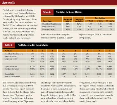
All variables used in the following analysis are stochastic and assumed to be log-normally distributed. For replication purposes, means and standard deviations in the model can be set as desired. In this paper, it is estimated that: (1) future annual home appreciation will be 3.0 percent with a 5.0 percent standard deviation; (2) that the one-month LIBOR will average an annual rate of 2.07 percent (currently it is less than 0.25 percent) with a 0.53 percent standard deviation; and (3) that annual future inflation (CPI–U) will average 2.50 percent with a 1.32 percent standard deviation.

Future portfolio returns are based on forecasts of future asset class risks and returns as described by Michaud, Michaud, and Balter (2013). In the model, the expected future return on long-term fixed income securities is 3.8 percent with a 10.1 percent standard deviation. The security market line ranges up to an expected future return of 8.0 percent on a portfolio that is 100 percent in equities having a standard deviation of 16.0 percent. These are nominal, not real returns. If future inflation averages 2.50 percent per year, the real return on equities would be 5.5 percent and the real return on fixed income would be 1.3 percent. These figures are similar to the real returns on equity and fixed income used in Finke, Pfau, and Blanchett (2013). Pfau (2012) has an extensive literature review on safe withdrawal rates. The model portfolios used in the simulations are shown in Table 3 in the appendix.

Given one portfolio, one desired first-year draw rate, and one spending horizon, 2,000 Monte Carlo simulations were run across seven options. The first used the portfolio only with no reverse mortgage. The next six were various plans using the HECM. The various reverse mortgage plans are discussed below. For each of the 2,000 separate runs, four Monte Carlo arrays, 50 years in length, were created and used in calculating all seven options. One array is the portfolio return; others are one-month LIBOR, inflation, and home appreciation. The 2,000 results are tabulated at the spending horizon. Data are also tabulated at an intermediate year as few retired people remain in their home for 30 years.

Across eight initial withdrawal rates ranging from 3.0 percent to 6.5 percent, across eight portfolios with equity exposure from 20 percent to 100 percent, and over two spending horizons (30 years and 37 years), the seven options required 896 Monte Carlo runs, each with 2,000 iterations (each iteration required 20,000 formulas).

First, the 4 percent rule was tested to determine how it and other withdrawal rates succeed across various portfolio asset allocations. Portfolios that have equity exposure of 60 percent and higher reach close to or exceed the 90 percent success level if the initial withdrawal rate is 3.75 percent, not 4.0 percent. Portfolios with less than 60 percent equity exposure have success levels commensurate with their equity exposure. The withdrawal rate success of portfolios with equity exposure of 60 percent and higher converge near the 90 percent success rate level. The extra volatility of the 100 percent equity portfolio makes its chances of success no better than the 70 percent equity and 80 percent equity portfolios.

In testing, it was shown that a portfolio that is 60 percent in equities has only a 36 percent chance of withdrawal success if the initial withdrawal rate is 6.0 percent and grows, on average, by 2.5 percent each year. It will now be shown that a 6.0 percent withdrawal rate can exceed 90 percent success with the use of a reverse mortgage as a portfolio supplement.

Supplementing Portfolio Withdrawals with a HECM Reverse Mortgage

Six ways of accessing funds from a reverse mortgage, across a spending horizon of 30 years, were examined for a 63-year-old borrower living in a $450,000 home and having an $800,000 retirement portfolio. The first year’s desired withdrawal is 6.0 percent, which is $48,000. This is equivalent to $4,000 per month. After paying federal and California taxes, this leaves the homeowner with $2,583 to spend. The six HECM reverse mortgage possibilities are as follows:

Tenure Advances: A tenure advance lasts as long as the home is the borrower’s primary residence. With the HECM, the monthly amount is calculated as a term loan to age 100. For the 63-year-old borrower, that is 444 months, producing $1,328 tax-free each month from the HECM. On a tax equivalent basis, that is $2,057, so to meet the desired portfolio withdrawal of $4,000, only $1,943 needs to be withdrawn from the portfolio each month during the first year. Because the HECM tenure advance is fixed, the monthly portfolio withdrawal in the second year will be $2,043. The $100 increase over the first year accounts for the 2.5 percent expected annual inflation.

Term Loan Advances Over the Spending Horizon: This withdrawal approach changes the monthly advance calculations to 360 months. The result is $1,412 distribution, which has a tax equivalent value of $2,187. So, over the first year only $1,813 needs to be withdrawn each month. Because the HECM term advance is fixed, the monthly portfolio withdrawal in the second year will be $1,913 to account for the 2.5 percent inflation.

Term Loan First: This approach means setting up tax-free monthly HECM withdrawals of $2,583 so the portfolio need not be touched. It works out that a HECM can provide this level of distribution for 118 months before its capacity is exhausted. Because the HECM term advance is fixed, the monthly portfolio withdrawal in the second year will be $100 higher to account for the 2.5 percent inflation. With the term loan first option, the portfolio can grow with only minimal withdrawals for 9.4 years. After that time, 100 percent of the spending money must come from the portfolio.

Line of Credit Draws First: This method is discussed by Sacks and Sacks (2012). For example, $2,583 is drawn from the HECM line of credit each month during the first year, and $2,647 is drawn from the line of credit each month during the second year. A similar progression occurs each subsequent year. These withdrawals, growing each year with inflation, continue until the HECM is exhausted. The portfolio can remain untouched over this period. However, as will be shown, this “line of credit draws first” option is dominated by the “term loan first” option owing to the method HECM uses to find scheduled monthly loan advances.¹

Line of Credit Draws with a Fixed Threshold: This approach requires a fixed threshold to be selected, such as 5.0 percent. This means that if the portfolio’s return last year was less than 5.0 percent, the borrower should make the entire after tax monthly withdrawal from the HECM line of credit. In this example, the homeowner should withdraw $2,798 tax-free and not touch the portfolio. However, if the portfolio return was better than 5.0, percent, the borrowers should make the entire monthly withdrawal from the portfolio, which would be $4,000 taxable (and not touch the HECM). Twenty thresholds of annual portfolio returns ranging from +90 percent to –90 percent were tested. In the Monte Carlo runs, an annual portfolio return of +90 percent was never reached, so the results are the same as HECM “line of credit draw first.” A –90 percent threshold (that is minus 90 percent in one year), is always surpassed, so the portfolio is always drawn first, and the HECM line of credit would be accessed only if and when the portfolio is depleted.

Sacks’ Coordinated Strategy: This strategy (Sacks and Sacks 2012) consists of portfolio draws only from annual positive portfolio returns. Any shortfall in the desired annual withdrawal is made up by drawing on the reverse mortgage line of credit. When the reverse mortgage line of credit is exhausted, all withdrawals are made from the portfolio regardless of its annual returns.

Figure 1 plots success rates for these reverse mortgage options across various portfolios. Portfolios that are 60 percent or more invested in equities are very successful in meeting desired withdrawal requirements. With 60 percent invested in equities, the chances of spending success for these portfolios range from 86.8 percent for the “line-of-credit draw first” option up to 92.2 percent for the “term loan advances to spending horizon” option. With this option, loan advances stop at the end of 30 years, hence, it surpasses the “tenure advances” option. That is because tenure advances are calculated to when the borrower will reach age 100. In this case, that is 37 years. However, tenure advances continue indefinitely, even if the homeowner lives to be 110. Using a 30-year spending horizon, no credit is given for those extra advances.

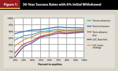
If success over a spending horizon is all that matters, Figure 1 shows that the success rate increases only marginally as the portfolio is invested in more than 70 percent equities. Bengen (1994, p. 179) stated that “Stock allocations below 50 percent and above 75 percent are counterproductive.” It appears that he may be correct.

Thirty-year success rates are important to give clients a sense that their retirement planning is sound. In this study, average portfolio balances, home values, and loan balances have been calculated at 30 years; but 30 years is a long way off. As abundantly pointed out in the literature, if spending withdrawals are successful over 30 years, there may be millions of dollars left on the table. More meaningful results would be those at some intermediate period, say 15 years.

Figure 2 shows the retiree’s expected net worth at the end of 15 years. This is the total of their expected portfolio balance and their remaining home equity. With the “portfolio only” (no reverse mortgage) option, the home equity is the entire future home value. Obviously, the highest portfolio balances result in the two options where the reverse mortgage is drawn first and the portfolio is allowed to grow with little or no withdrawals for much of the 15 years. The lowest two portfolio balances among the reverse mortgage options are those where the line of credit is used only intermittently. The less a reverse mortgage is utilized, the more is drawn from the portfolio, and hence, the lower the portfolio balance. Greater utilization of the reverse mortgage gives higher portfolio balances, but necessarily uses up home equity. The six reverse mortgage options give higher overall results across all portfolio equity mixes than just relying on the portfolio as the source of retirement spending.

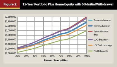
Two reverse mortgage strategies dominate. Which one to choose depends on a client’s comfort level in using home equity to supplement portfolio withdrawals. One strategy is reverse mortgage first. The “term plan first” plan dominates the “line of credit first” plan in both withdrawal success and expected net worth. If the portfolio is invested 70 percent in equities, the “term plan first” plan would give an 89.4 percent chance of withdrawing 6.0 percent annually over 30 years (rising with inflation), versus a 42.8 percent chance that the portfolio, going it alone, could give these desired withdrawals, and, at 15 years, a client’s net worth could be $429,500 higher.

The second strategy is reverse mortgage “term advances over the spending horizon.” Expected net worth is less than the first strategy, but at 15 years the loan balance is smaller, and the 30 years spending success rate is several points higher. If the portfolio is invested 70 percent in equities, the “term advances over the spending horizon” plan would give a 93.2 percent chance of success of withdrawing 6.0 percent annually over 30 years (rising with inflation), and, at 15 years, a client’s net worth could be $282,800 higher.

Mortality Issues

Generally, a client must plan ahead longer than one thinks. The previous notes were calculated over a 30-year spending horizon. It is important that clients realize that life expectancy is a median (there is a 50 percent chance that they will live past their life expectancy). Say that Marilyn is a 63-year-old female in excellent health and her life expectancy is 24.8 years. This means there is a 50 percent chance that she will live to be 88 years or older. If her health was only average, Marilyn would have a 50 percent chance of living to age 84 or older.²

Her husband George is a 65-year-old male in excellent health with a life expectancy of 20.4 years. This means there is a 50 percent chance that he will live to be 85 or older. If his health was only average, George would have a 50 percent chance of living to age 81 or older. Given that they are both in excellent health, there is a 68 percent chance that Marilyn will outlive George. At his life expectancy, she will be 83 and could expect to survive an additional 8.5 years (again a median figure). There is a 32 percent chance that George will outlive Marilyn. At her life expectancy, he would be 90 and could expect to survive her by 4.9 years. There is a 50 percent chance that at least one of them will be alive in 28.6 years. This is known as a last-to-die joint life expectancy.

With a 30-year spending horizon, annuitant mortality tables indicate the probabilities that: there is a 5.1 percent chance that both be will alive, and 42.2 percent chance that someone will be alive. So, if planning over only 30 years, there is a 42 percent chance that at least one of them will outlive their money. To be prudent, it would be safer to choose a planning horizon where there is only a 10 percent chance that someone is still alive. With Marilyn and George, the nearest full year that gives close to a 10 percent probability is year 37, where there is an 11.6 percent chance that someone is still alive.

Planning over a 37-year period eliminates the advantage of the “term to horizon” reverse mortgage advance option. This is because the HECM “tenure advance” is calculated to a point when the younger borrower reaches age 100; yet, the monthly advances continue indefinitely. In this example, a 37-year “term to horizon” plan would result in the same monthly advance dollars, but the term advances would stop when the younger borrower reached age 100.

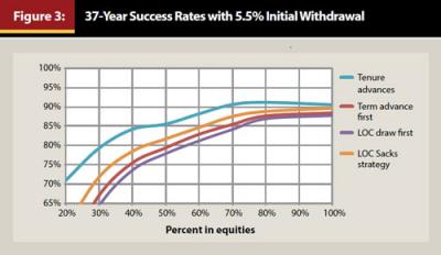
Over 37 years, the portfolio alone can only support a 3.25 percent first-year withdrawal if the expected failure rate is not to exceed 10 percent. This is possible with portfolios that are 70 percent or more invested in equities. Figure 3 shows that the first-year withdrawal can safely be increased to 5.5 percent with a reverse mortgage supplement. This is 62 percent higher annual spending in retirement when compared to the 3.25 percent that the portfolio going it alone could provide.

The expected portfolio balance will obviously be higher in 15 years if a reverse mortgage is used to supplement portfolio withdrawals, but home equity will be lower as funds are withdrawn from the reverse mortgage. As seen in Figure 4, the total of the portfolio balance and the home equity will be materially higher at 15 years when a reverse mortgage is used as a portfolio supplement.

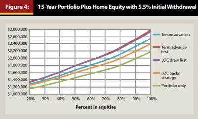
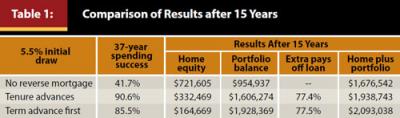
Again two reverse mortgage strategies dominate. One strategy is a reverse mortgage “home tenure” plan. Expected net worth is less than the “term first” strategy, but at 15 years the loan balance is smaller, and the 37-year spending success rate is several points higher. If the portfolio is invested 70 percent in equities, the “home tenure” plan would give a 90.6 percent chance of withdrawing 5.50 percent annually over 37 years (rising with inflation), and, as shown in Figure 4 at 15 years, your client’s net worth could be $262,000 higher.

The second strategy is reverse mortgage first, and the “term plan first” plan dominates the “line-of-credit first” plan in both withdrawal success and expected net worth. If the portfolio is invested 70 percent in equities, the “term plan first” plan would give a 85.5 percent chance of withdrawing 5.50 percent annually over 37 years (rising with inflation), versus a 41.7 percent chance that the portfolio, going it alone, could give these desired withdrawals, and, as shown in Figure 4, at 15 years your client’s net worth could be $416,500 higher.

Table 1 recaps the simulated results if the portfolio is invested 70 percent in equities. Of interest is the chance that the extra portfolio balances resulting from the reverse mortgage supplements can, after being disbursed and paying taxes, have a very good chance of paying off the loan.

Planning In a Low-Yield World

Using recent market conditions as predictors, rather than historical security returns, Finke et al. (2013) suggest that 2.5 percent may be the new SAFEMAX withdrawal rate. Using the Finke et al. future market conditions as inputs, this analysis found a 92.5 percent chance of spending success over 30 years with an initial withdrawal of 2.5 percent. With a 4.0 percent initial withdrawal, the portfolio alone has only a 73.1 percent chance of spending success; adding reverse mortgage options raised success rates to between 98 and 99 percent. Additionally, with a 5.0 percent initial withdrawal, the Finke et al. portfolio alone has only a 51.7 percent chance of success; adding reverse mortgage options raised spending success rates to between 89 and 92 percent.

Using a 5.0 percent versus a 2.5 percent initial withdrawal rate indicates that a client can double expected spending over a 30-year retirement horizon by adding a reverse mortgage supplement. At 15 years, the extra net worth with the reverse mortgage options ranged from $181,000 to $364,000. So, if one believes that a low yield world is likely in the future, reverse mortgages can play a role even more decisive than that expressed in the bulk of these notes.

Relative Home/Portfolio Values

The benefits of using a reverse mortgage will vary depending on the relative initial values of the portfolio and the home. The examples shown in this paper are based on a $450,000 home and an $800,000 portfolio. The monies available from a reverse mortgage are based on home values, so the larger the home value with respect to the portfolio, the greater the relative benefit from a reverse mortgage.

The examples show that the 37-year success rate of a 5.5 percent initial withdrawal is between 86 and 91 percent. If the home was valued at $250,000, rather than $450,000, the initial withdrawal rate would have to be reduced to 4.5 percent to have between an 88 and 90 percent success rate. But this is still clearly better than the 37-year, 3.2 percent withdrawal rate which the portfolio, without a reverse mortgage, could supply. If the home is valued at $250,000, rather than $450,000, the 15-year increase in net worth compared to a “no reverse” strategy is still between $138,000 and $241,000.

Downsides of a Reverse Mortgage

It is important that financial planners and their clients fully understand the costs associated with reverse mortgages. Many consumer advocates believe that these products are highly priced and lack appropriate disclosure. As such, it is imperative that financial planners engage in high level due diligence before incorporating the strategies presented in this paper into plans for clients. Additionally, the traditional American borrower has been a “house rich and cash poor” senior. If a borrower struggles to manage their money, they might spend it too quickly and have no nest egg left. Others may go into default and face possible foreclosure for not keeping their property taxes and homeowner’s insurance current. Others might be duped by those cross selling financial products. If a planner suspects that any of these factors are present with a client, the use of a reverse mortgage should be thoroughly reviewed.

Summary

Today, very few Americans in retirement or about to retire have entered into a reverse mortgage. Some clients will resist the use of these products because they consider their home as sacred. However, a reverse mortgage may be considered as another financial planning tool with no stigmas attached to its use. As this paper highlights, reverse mortgages offer many benefits, such as:

• Tax-free advances that are guaranteed by HUD, and unlike a home equity line of credit cannot be arbitrarily cancelled;
• The annual tax-free advances can be 3.52 percent (over 37 years) or 3.74 percent (over 30 years) of the home’s current value;
• The annual portfolio withdrawals can thus be smaller or delayed;
• The extra portfolio balance will often be greater than the loan balance in 15 years;
• Depending on the relative values of the home and portfolio, withdrawal rates of 5.0 percent to 6.0 percent can be achieved with over a 90 percent chance of success over 30 years; and
• In a low yield world, a reverse mortgage supplement has an even greater impact on “spending success.”

 

Endnotes

1. The note rate on a HECM varies each month based on the one-month LIBOR plus a set lender’s margin. The HECM pricing model uses the 10-year LIBOR swap rate as a proxy for the next 120 months of the one-month LIBOR. Adding the lender’s margin, this 10-year rate is called the expected rate. Advances under term and tenure payment plans are calculated using this expected rate plus the 1.25 percent MIP, but the line of credit grows only at the current one-month LIBOR plus margin plus the 1.25 percent MIP. Think of a car loan; higher rates mean higher payments. That is why HECM scheduled payment plans dominate line-of-credit advances. For example, assume that, after costs, $229,100 is available from a HECM reverse mortgage and that the spending horizon is 30 years. If the 10-year swap rate is 2.81 percent and margin is 2.25 percent, then the expected rate is 5.06 percent. A 30-year term plan would give $1,412.13 each month. If the one-month LIBOR is 0.20 percent and the margin is 2.25 percent, the note rate is 2.45 percent. So steady line-of-credit draws could amount to only $1,051.27 each month. Thus, with today’s rates, a term plan can pay out 34 percent more than a line-of-credit plan. An inverted yield curve would reverse this effect. Because the current one-month LIBOR is historically low, simulations use 2.07 percent, the average for the last 10 years. Readers should note that the monthly average for the one-month LIBOR for September 2008, when Lehman Brothers fell, was 2.93 percent, and by January 2009, the monthly average had dropped to 0.38 percent. In October 2013, it is down to 0.17 percent.
2. For individuals in excellent health, 1996 U.S. Annuity 2000 tables (as published by the Society of Actuaries) were used. For individuals in average health, general population U.S. Decennial Life Tables (as published by the National Center for Health Statistics) were used.

References

Bengen, William. 1994. “Determining Withdrawal Rates Using Historical Data.” Journal of Financial Planning 7 (4): 171–180.

Bierwirth, Larry. 1994. “Investing for Retirement: Using the Past to Model the Future.” Journal of Financial Planning 7 (1): 14–24.

Cooley , Philip L., Carl M. Hubbard, and Daniel T. Walz. 2011. “Portfolio Success Rates: Where to Draw the Line.” Journal of Financial Planning 24 (4): 48–60.

Finke, Michael, Wade D. Pfau, and David M. Blanchett. 2013. “The 4% Rule Is Not Safe in a Low-Yield World.” Journal of Financial Planning 26 (6): 46–55.

Michaud, Richard, Robert Michaud, and Daniel Balter. 2013. “fi360 Asset Allocation Optimizer: Risk-Return Estimates.” Boston: New Frontier Advisors LLC. www.flexscore.com/ui/content/CapitalMarketInputs.pdf.

Pfau, Wade D. 2012. “Capital Market Expectations, Asset Allocation, and Safe Withdrawal Rates.” Journal of Financial Planning 25 (1): 36–43.

Sacks, Barry H., and Stephen R. Sacks. 2012. “Reversing the Conventional Wisdom: Using Home Equity to Supplement Retirement Income.” Journal of Financial Planning 25 (2): 43–52.

Salter, John, Shaun Pfeiffer, and Harold Evensky. 2012. “Standby Reverse Mortgages: A Risk Management Tool for Retirement Distributions.” Journal of Financial Planning 25 (8): 40–48.

Scott, Jason S., William F. Sharpe, and John G. Watson. 2009. “The 4% Rule - At What Price?” Journal of Investment Management 7 (3). www.stanford.edu/~wfsharpe/retecon/4percent.pdf.

Stout, R. Gene. 2008. “Stochastic Optimization of Retirement Portfolio Asset Allocations and Withdrawals.” Financial Services Review 17 (1): 1–15.

Citation

Wagner, Gerald C. “The 6.0 Percent Rule.” Journal of Financial Planning 26 (12): 46–54