Transition Through Old Age in a Dynamic Retirement Distribution Model

Journal of Financial Planning: December 2012

Executive Summary

• Past research on the topic of sustainable withdrawal rates has primarily focused on longer distribution periods that apply to younger retirees.
• This research project seeks to answer the following questions regarding superannuation (continuing to survive and live into very old ages):
  -   What does the withdrawal rate profile need to look like for a retiree who survives into extreme old age?
  -   What should the withdrawal rate sequence be to sustain portfolio values sufficient to continue cash flows from old retirement ages throughout superannuation?
• Sequence risks, distribution periods (longevity percentiles), asset allocations, and superannuation represent the factors incorporated into four “levers” to measure and manage sustainable distributions from the earlier retirement years through superannuated retirement ages.
• Equity allocations above 50 percent cause an “allocation volatility drag” on optimal withdrawal rates.
• High cash flows early in retirement deplete portfolio values and reduce cash flows during later retirement years. How does a practitioner measure this effect to manage cash flows for the present and future?
• Dynamic, serially connected, and annually recalculated cash flows based on age and longevity percentiles provide insights into retirement distribution tradeoffs.
• This paper develops a “longevity-based methodology” to rationally restrain the early age withdrawals to improve portfolio survivability later in retirement with transition between the two stages in the mid-70s.

Larry R. Frank Sr., CFP^®, is a registered investment adviser with an M.B.A. from the University of South Dakota. He lives in Rocklin, California. (LarryFrankSr@BetterFinancialEducation.com) 

John B. Mitchell, D.B.A., is professor of finance at Central Michigan University. His research focuses include simulation-based retirement planning models, the statistical properties of financial time series, assessment of learning, and derivatives strategies. (mitch1jb@cmich.edu)

David M. Blanchett, CFP^®, CLU, AIFA^®, QPA, CFA, is head of retirement research for Morningstar Investment Management in Chicago, Illinois. He has published more than 30 papers in various industry journals. (david.blanchett@morningstar.com)

This paper extends the three-dimensional (3-D) distribution model developed in the work of Frank, Mitchell, and Blanchett (hereafter FMB) (2011 and 2012) by demonstrating the adjustment of withdrawal rates to reduce the risk of ruin caused by superannuation (continuing to survive and live into very old ages).

A structural problem with pensions, immediate annuities, and first generation “safe withdrawal rates” is a disconnect between the benefits paid and the underlying asset values required to support those promised benefits. Underlying asset values are variable and may decrease in value, temporarily or permanently, because of market or spending forces, while payments are often fixed or include a cost-of-living adjustment upward. A divergence between payments and asset values may not be sustainable.

Assurance against superannuation usually involves forgoing consumption at earlier ages to maintain reserves for consumption during later years. This paper proposes a self-managed process and lays out a withdrawal rate methodology to smooth the transition from the earlier retirement years into old age. Alternatively, retirees can buy annuities at the cost of a loss of control over at least a portion of their wealth. This paper presents an alternative to that loss of control that retirees can use to make decisions about how to manage the risk of superannuation and retain assets for subsequent consumption and bequest.

FMB 2011 and 2012 describe, in a 3-D model, how to simultaneously measure and incorporate three methodological adjustments to refine and measure: (1) market returns (sequence risk as measured by probability of failure (POF)), (2) longevity risk (impact of strategic use of longevity percentiles on the distribution period), and (3) asset allocation (effect of allocation on withdrawal rate). This paper adds a fourth methodology adjustment to the 3-D model to address superannuation risk, the risk that the retiree continues to live into very old ages.

Withdrawal rates (one dimension in the 3-D model) are most sensitive to two fundamental factors, the distribution period (DP) (age, the second dimension) and the market returns. FMB 2012 demonstrated that longevity risk affects the distribution period, which is the primary factor that determines the withdrawal rate. The effects of variable market returns (commonly referred to as sequence risk) may be measured by the POF.¹ FMB 2011 demonstrated that withdrawal rates have an associated POF that can be used to measure the impact of market declines or gains on portfolio values. How do retirement planners separate these two components (DP and sequence risk) when helping retirees make decisions about the sustainability of their distributions?

To complicate matters, a third factor, asset allocation (illustrated in FMB 2011 as the third dimension), also affects withdrawal rates, although to a much lesser extent than most imagine.

Methodology, Longevity, and Asset Classes

The use of serially connected, annually recalculated life expectancy and the use of longevity percentiles to determine the current DP as the retiree dynamically ages was developed and presented in FMB (2012). Longevity percentiles (LP) determine how long the distribution period is in the remaining life distribution. A low LP (fewer people outlive) results in a longer DP, and vice versa. Returns are based on five asset classes from January 1926 until December 2010. All returns are converted into “real returns” (adjusted for inflation), where inflation is defined as the increase in the Consumer Price Index for Urban Consumers, data obtained from the Bureau of Labor Statistics.

This paper replicates FMB 2012 with respect to joint ages, life table, asset allocation, portfolio starting values, longevity percentiles, and probability of failure (and is fully comparable to the authors’ working paper FMB 2012 SSRN). The only methodology adjustment in this paper is applied to the withdrawal rate and the use of both the Social Security Period Life Table and Society of Actuaries Annuity 2000 Mortality Table. As a reminder to the reader, returns and cash flows are expressed in real terms.

Because the expected remaining distribution periods become quite short at older ages, the corresponding withdrawal rate for each DP grows very high. The unadjusted withdrawal rate increases exponentially because of this shrinking period effect. In this paper, the withdrawal rate is adjusted through WR percent*(1/n), where WR percent represents the withdrawal rate for the current dynamically recalculated DP, and n equals the number of years remaining in the DP. n = DP = age_LP minus age_current, where LP = longevity percentile-derived possible age of death, and current = retiree present age.

For example, if WR percent = 3.97 and if n = 20, the adjustment to WR percent is 1/20 or (.05)*0.0397 = 0.001985. Thus the adjusted WR percent is 0.0397 – 0.001985 = 0.037715, or 3.77 percent. As n decreases due to shorter longevity, the value for (1/n) increases, which increasingly reduces the WR percentage.² See an example below in Practical Applications, step four. As n decreases due to shorter longevity, e.g., 10 years remaining longevity and then five years remaining, the value for 1/n increases: 1/10 = .10 (10 percent) and 1/5 = .20 (20 percent). This paper addresses this problem of growing percentage withdrawals, which means more rapid depletion of the portfolio balance, by introducing the method to dampen the effect of shorter distribution periods.

Phase I uses the Social Security longevity tables (2007)³ because this data represents the general population and is also the same table used in FMB (2011, 2012)—thus, a direct extension and comparison of the three-dimensional work to demonstrate how this methodology transitions a retiree from younger retirement years into superannuated retirement years.

Phase II applies the 3-D model and this paper’s methodology to the Annuity 2000 tables⁴ to apply this methodology to that “healthier” population segment who are more likely to be interested in superannuation management of withdrawal rates (Krueger 2011).

Retiree Outlooks

There are two types of retiree outlooks: (1) the desire to consume a bit more during their early “go-go” years and cut back during their “slow-go” and “no-go” years (called “consumption-oriented” in FMB 2012) (Stein 1998), and (2) those who may recognize, or worry about, longevity due to family history, and thus prefer to “push” their consumption into later years by preserving some of their current portfolio balances (called “inheritance-oriented” in FMB 2012). Arguably, the retiree who begins as consumption-oriented must switch to less consumption at some point to preserve portfolio balances.

The problem with consumption orientation is that portfolio balances are spent early. At what age should a retiree change their consumption pattern? At what age do retirees begin to recognize they may continue to live into very old ages? A transition in thinking may occur at any age; however, the earlier the better, because success depends on retaining portfolio balances in earlier years for subsequent use in later years.

FMB 2011 and 2012 demonstrated the use of annually recalculated longevity percentiles to determine the potential remaining number of years in a retiree’s lifetime, which then equates to the length of the distribution period, to distinguish between a bequest-oriented retiree⁵ (low longevity percentile value: one who wishes some consumption from their portfolio, but also to pass on as much of it as feasible) and a consumption-oriented retiree (high longevity percentile value: one who wishes to maximize consumption early with less emphasis on providing a bequest later). A low longevity percentile (for example, 10th percentile) age results in a longer DP because fewer cohorts survive to that age by definition. A high longevity percentile (for example, 75th percentile) results in a shorter DP because more cohorts survive beyond this DP definition (FMB 2012). Therefore, bequest-oriented withdrawal rates are lower than consumption-oriented withdrawal rates, illustrated in Figure 1 as unadjusted strategies. Both lines converge at age 95 because the LP percentiles, thus the DP, converge by methodology design in FMB 2012.

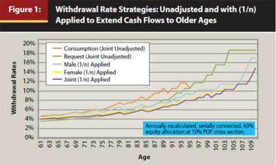
Notice also in Figure 1 that the elderly (late 80s plus) unadjusted withdrawal rates become quite large—over 10 percent. A high withdrawal rate begins to cause problems for those who continue to live into older ages because their portfolio values deplete faster, resulting in lower relative cash flows from lower portfolio values during these later years. This impact is discussed in greater detail later in the paper.

This paper develops a “longevity-based methodology” to rationally restrain the early age withdrawals to improve portfolio survivability later in retirement. The method consists of serially connected, annually recalculated life expectancy and use of longevity percentiles to determine the current DP as the retiree dynamically ages to replicate real life. The withdrawal dollar amount adjustment is longevity based because the higher withdrawal rates result from ever-shorter distribution periods that come from shorter lifespans at older ages and incorporates current age as a main point of reference to establish the DP.

This paper develops a method to ration­ally (as opposed to ad hoc) restrain withdrawal rates for the retiree who desires to measure and monitor elderly cash flow maintenance in case he or she (or they) continue to live into very old ages. For such elderly ages, distribution periods become quite short because of shortened expected longevity, which results in high withdrawal rates. This paper also seeks to determine at what age, or age range, retirees should begin to implement transition to a superannuation plan as proposed below.

Figure 1 clearly shows that the consumption-oriented retiree withdrawal rates remain quite high throughout this retiree’s lifetime. The effect, shown later in Table 1, is a reduction of portfolio values early in retirement that results in reduced cash flows from those subsequent lower portfolio values. At the other end of the withdrawal spectrum is the bequest-oriented retiree with lower withdrawal rates. These lower withdrawal rates retain portfolio values better relative to the other strategies up to the late age 70s, at which point the (1/n) adjustments for female and joint retirees are lower. This suggests that retirees should switch from either consumption or bequest orientation to a “preservation orientation” at an age when the retiree has transitioned to worrying about outliving their money.

Retirees may have a consumption-oriented goal during their young retirement years, as illustrated in Figure 1. However, practitioners and retirees alike should understand that adjustments first toward bequests and subsequently toward sustaining cash flow into very old age (because the retiree continues to survive) need to be considered, especially in their “mid-retirement years” of mid- to late 70s. Retirees with an original bequest-oriented goal (they started with lower longevity percentiles to extend the distribution periods at a young retirement age, therefore having lower withdrawal rates) do not need to make this adjustment until approximately half a decade later (early 80s).

Third Dimension: Asset Allocation

One of the “levers” that may be used by retirees to monitor their exposure to the probability of failure of their withdrawals is a result of their asset allocation. Figure 2 illustrates the impact of various equity allocations on a sustainable withdrawal strategy, the third dimension (FMB 2011, 2012). The 60 percent equity line in Figure 2 corresponds to the “Joint 1/n Applied” line in Figure 1 as a point of reference. Notice the close clustering around equity allocations less than 50 percent. (Peak withdrawal rates of various allocations, derived from this methodology, are highlighted in Appendix F of FMB 2012 SSRN. These results compare to a degree to those in Pfau 2012). Graphed lines are not “smooth” due to rounding of distribution periods derived from changing longevity percentiles with age.
 

There exists an asset allocation volatility drag on the withdrawal rate, which reduces the optimal allocation based on the distribution period. Data from Pfau and the authors’ research in FMB 2012 SSRN suggests that shorter distribution periods tend to have more optimal withdrawal allocations with less equity (volatility), and vice versa.

Social Security and Annuity 2000 Tables Compared

Before application of the Annuity 2000 table, it is instructive to look at the differences in DP between the two tables based on LP. The Annuity 2000 table is based on the longevity of “healthier” people (Kreuger 2011), thus the DPs would be expected to be longer than those from the Social Security table, which is based on the general population. But, how much of a difference is there between tables? Is it consistent across longevity percentiles and ages?

FMB 2012 SSRN shows a complete comparison of DP differences between the two tables at various LPs. In summary:

• At the 20 percent LP (longer DP compared to expected longevity), the annuity table DP is approximately four years longer than the Social Security table DP up to age 90, then three years longer to age 98, two years to age 103, one year to age 106, and then the tables converge at higher ages
• At the 50 percent LP (expected longevity), the annuity table DP is four years longer to age 68, three years to age 80, two years to age 98, one year to age 103, and then the tables converge
• At the 80 percent LP (shorter DP compared to expected longevity), the annuity table DP is four years longer to age 63, three years to age 67, two years to age 78, one year to age 99, and then the tables converge

Distribution period differences tend to be greater, and last longer, for lower LPs. The Annuity 2000 table, where people are healthier than the general population, combined with LPs less than 50 percent (longer longevity than expected), leads to an “inheritance orientation” (FMB 2012), which conserves resources for retirees to use should they continue to live and need the resources, facing the risk of superannuation.

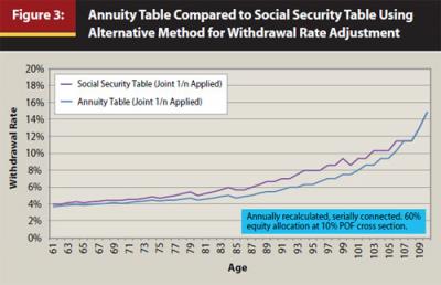
The DP affects the withdrawal rate directly—longer DPs (Annuity 2000 table) have lower withdrawal rates compared to the Social Security table, and vice versa, as shown in Figure 3. Do these lower Annuity 2000 table withdrawal rates result in cash flow differences?
 

The left half of Table 1 illustrates the cash flow and terminal portfolio value differences between the annuity table and Social Security table using this paper’s adjusted methodology. The percentiles represent Monte Carlo simulation percentiles where the 5th (best one in 20) and 25th (best one in 4) percentiles represent the “good” market sequence cash flows and the 75th (worst one in four) and 95th (worst one in 20) percentiles represent the “bad” market sequence cash flows. The right half of Table 1 illustrates these same values from the consumption-oriented retiree in FMB 2012 and graphed in Figure 1. The data for the upper half of Table 1 are derived from 30 percent target POF (FMB 2011 and 2012), while the lower half of Table 1 targets 10 percent POF values. Withdrawal rates would be higher for the upper half relative to the lower half, and higher for the right half relative to the left half. These right and left halves compare the consumption versus superannuation strategy results, while the top and bottom halves compare the differences between using higher or lower target POF (sequence risk, FMB 2011).

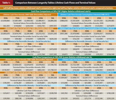
The debate then turns to consideration of just how healthy does the retiree think he or she is, because the annuity table difference is derived from supposedly healthier people (due to the adverse selection issues associated with annuity purchases). Clearly, Table 1 demonstrates the advantage of reducing withdrawal rates for bequest and preservation (left half) when compared to the consumption-oriented retiree (right half).

The differences between lifetime withdrawals are small, although the results favor slightly lower withdrawal rates in general; in other words, the annuity table in both cases. The fundamental goal (left half of Table 1) is the desire to retain portfolio balances to sustain higher cash flows during later years. The alternative is to pull cash flow into early retirement years (right half of Table 1) and thus reduce portfolio values such that cash flow in elderly years must be reduced. Lifetime cash flow results are very similar between tables; however, higher consumption in early years, regardless of table, results in a reduced lifetime cash flow and terminal values (right side of table). Once a dollar has been consumed, that consumed dollar’s growth potential is also consumed, reducing future cash flow potential. The question remains, at what age is cash flow into later ages a concern for the retiree? The answer: late 70s or early 80s, as discussed below.

The primary differences between quadrants come from differing DPs that result from using the different life tables as well as higher (consumption) or lower (superannuation) longevity percentiles of either life table. Using both POF and longevity percentiles in unison allows measurement to expose tradeoffs between cash flows and terminal value impact.

Incorporating Sequence Risk Measures

Most retirees prefer an established, fixed monthly withdrawal dollar amount as opposed to a variable dollar amount that changes each quarter or monthly. The fixed dollar amount may be adjusted up or down annually or more often should markets deteriorate sufficiently.

The cash flows and portfolio balances are annually recalculated and serially connected to reflect real life. The reader may be tempted to interpret percentiles in Table 1 as predictive. However, no one knows if the retiree is on a “successful” track (percentiles greater than 50 percent) or “unsuccessful” track (percentiles less than 50 percent) unless the retiree also evaluates their probability of failure (FMB 2011). Stated another way, the cash flows are from results internal to simulations. Cash flow percentiles are market related and beyond retiree control. The reader may think market returns may be controllable through asset allocation, however, Figure 2 suggests otherwise.

A retiree’s actual, real-life, distribution path would be transient, crossing among simulated paths because of actual market results they experience as well as withdrawal decisions they make over time.

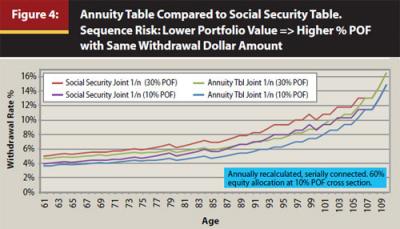
Figure 4 illustrates the situation where portfolio values have declined such that the withdrawal rates reach their corresponding 30 percent POF values based on fixed withdrawal dollar amounts established using the 10 percent POF withdrawal rate. FMB 2011 found that as the withdrawal rates go up to reach 30 percent POF rates, the retiree should consider retrenching spending because this is a signal that the dollar amounts withdrawn may be becoming unsustainable given current market conditions. FMB 2011 found this consistent across portfolio allocations.
 

The Table 1 discussion demonstrates that higher withdrawal rates deplete portfolio values faster, which leads to lower lifetime total cash flows and lower terminal values. The same effect would occur when higher POF rates are experienced for extended periods. Counter to intuition, higher withdrawal rates lead to lower lifetime withdrawals (compare the upper half (30 percent POF) to the lower half (10 percent POF) in Table 1) as a result of drawing down the portfolio early and therefore having a reduced portfolio balance from which to withdraw later. As expected, terminal values are lower with higher withdrawal rates.

Lower lifetime withdrawals extend portfolio values such that subsequent higher portfolio values at later ages may sustain higher dollar distribution amounts. This is an important consideration for those retirees who fear living into very old age. Use of POF informs the retiree whether their withdrawals put them in “good” (sustainable) or “bad” (unsustainable) profiles, either by market return sequences or by dollar withdrawal decisions or both.

How to Transition Between the “General Population” Table and the “Healthy” Table

Often it is difficult for retirees and practitioners to know during younger retirement years whether the retiree (individually or as a couple) will be favored by a longer-than-expected retirement. The shorter DP from using the general population (Social Security) table allows retirees during their “go-go” retirement years to have a higher withdrawal rate relative to the withdrawal rate derived from the longer DP of the “healthy” mortality table (Annuity 2000 table).

What are strategies a practitioner may use to transition retirees who begin to demonstrate a propensity for longer longevity (risk of superannuation)? Clearly, any strategy should consider how much of a withdrawal rate, and thus cash flow, adjustment should be made. This criterion suggests beginning to evaluate the superannuation possibility when the retiree is in their mid-70s. The first consideration is to switch to the Annuity 2000 table, if not already in use. The second consideration is to begin to use lower longevity percentiles when calculating the distribution period. The final consideration is to begin using the 1/n adjustment to the withdrawal rate to mute the exponential nature of growing withdrawal rates due to ever-shorter distribution periods related to older ages.

Practical Applications

It is not necessary to calculate or illustrate cash flows into the future to apply this model. Indeed, future return sequences are unknown, hence, it is unknown which cash flow percentile a retiree would actually follow in retirement. One may argue that the retiree most likely would experience multiple cash flow percentiles as they transition through the various market cycles during their retirement. Therefore, the following steps help evaluate, measure, and monitor a retiree’s sustainable cash flow.

The first step, selecting the portfolio asset allocation, has the smallest effect on the withdrawal rate (Figure 2) relative to the other steps. This step tends to maximize the withdrawal rate for a given POF.

The second step is to determine whether the retiree, if younger than 75, is consumption oriented or bequest oriented to determine a desired longevity percentile (FMB 2012). The LP determines the DP by subtracting the current age from a table-derived termination age. If 75 or older, low LPs may be desired since the retiree’s concern often transitions to even more concern of outliving their resources as they age. A low LP (low likelihood the DP would be outlived) results in a longer distribution period, thus a lower withdrawal rate percentage (FMB 2012). The LP thus determines the present year’s termination age from which to subtract the present year retiree’s age (age_Current) to derive the DP. AgeLP – age_Current = DP = n. Thus, for any age, the method to determine the LP and resulting termination age would be the same. The difference for older ages is the recognition of increasing risk that the retiree continues to age into even older ages (superannuation risk).

For those over age 75, the expression 1/n represents the inverse of the DP based on the number of years remaining for the LP of the retiree’s present age in step three. Recall that the methodology used here is annually recalculated, serially connected distributions for which one of the annually recalculated values is the DP. For practical reasons then, researchers and practitioners should become familiar with calculating LPs from the expected longevity period life tables to calculate the current DP for each retiree’s present age.

For example, in the case of joint lives, if the probability of a 65-year-old male living to age 85 is 40 percent and the probability of a 65-year-old female living to age 85 is 50 percent, the probability that either or both would live to that age would be 1 minus the probability that both are dead, which would be 70 percent (1 – ((1 – 0.4)*(1 – 0.5))); or alternatively, a 70 percent chance that at least one of the couple outlives age 85. Thus, the longevity percentile in this example is 70 percent for this 20-year (85 minus 65) DP. In this manner specific ages are combined with specific life expectancy to move away from generic distribution periods.

The third step is to decide on an initial POF. A low POF, such as 10 percent, provides a retiree with a lower fixed cash flow ability and allows the withdrawal rate to increase (decrease) with declining (rising) portfolio value due to market return sequences until a higher decision POF value is reached for spending retrenchment (FMB 2011). Alternatively, a fixed withdrawal rate (fixed POF) leads to a variable cash flow, which requires the retiree to have some flexibility with their spending. (See the Four “Levers” Summary below). Simulation software may be used, applying the DP from step two to determine the withdrawal rate that corresponds to the desired POF at the retiree’s current age.

The fourth step then applies 1/n to the withdrawal rate. This first adjustment applies an exponential character, because the growth in withdrawal rates has an exponential character (see Figure 1). For example, if the DP from above is determined to be 20 years, then 1/n = 1/20 = 0.05. 1 minus 0.05 = 0.95. If the unadjusted withdrawal rate = 5.29 percent, then the adjusted withdrawal rate for superannuation adjustment would be (0.95)(5.29 percent) = 5.02 percent; a slightly lower withdrawal rate to preserve the portfolio value for future distributions.

The superannuation adjustment in the methodology discussed in this paper, therefore, is to further extend DP and thus reduce the withdrawal rate further, through a progressively lesser longevity
percentile as the retiree ages. The resulting low LPs lead to a DP of such length that few may outlive it. Because the retiree has continued to survive, the risk becomes a probability the retiree may experience superannuation.

However, those who continue to survive are beating the probabilities of expected longevity (50th percentile), which requires using LPs that are less than 50 percent. LPs need to be reduced progressively to continue to extend the DP further. The fact that the retiree continues to live requires these adjustments because it is unknown just how long the retiree may continue to live.

An evaluation of any period life table demonstrates that the percentage of 90-year-olds, for example, surviving to age 100 is a higher percentage than 80-year-olds making it to age 100. Similarly, a higher percentage of 80-year-old cohorts will survive to age 100 relative to 60-year-old cohorts surviving to age 100. Therefore, closer attention to increased exposure to superannuation risk should be made for retires in their late 70s and early 80s. Even though the percentage of 60-year-olds living to 100 may be small, the odds of doing so increase simply by continuing to live. An adjustment mechanism needs to be developed to transition and manage portfolio balances for those who continue to live. Reducing the longevity percentile to 1 percent extends the distribution period by the maximum number of years remaining from the longevity tables.

The result is a more linear graph with a muted exponential character to reduce the withdrawal rate, thus extending portfolio values into the future, which mitigates the risk of superannuation.

Four “Levers” Summary

The three dimensions (time, allocation, and withdrawal rate), developed and illustrated in FMB 2011 and 2012, can be further refined and measured through the four levers summarized below. The 3-D model introduces cash flows that are dynamic, annually recalculated, and serially connected, including asset allocations, so that effects of prior decisions may be evaluated during retirement withdrawals. Past fixed-period-based research did not provide for the consideration of how time may be integrated into the decision-making process to measure and fully comprehend the effects of prior withdrawal decisions as well as effects of market return sequences.

Note that dynamic means a retiree starting retirement in their 60s may be consumption oriented, having a higher withdrawal rate that is measurable through methodology in FMB 2012. As the retiree ages into their late 70s, it may occur to them they may live longer than they initially thought, and begin to dynamically adjust their withdrawals to manage superannuation risk measurable through the methodology described in this paper. The retiree dynamically adjusts their withdrawal glide path profile through measureable processes that retain sustainable portfolio values for possible future years all through their remaining lifetime.

Now, however, the practitioner may better explain the tradeoffs and effects of various withdrawal glide paths on portfolio balances and how those future balances affect the withdrawal amounts. In other words, withdrawing higher amounts today equates to lower portfolio balances tomorrow. A retiree’s glide path is a result of prior decisions they’ve made, and one retiree’s glide path would be different from another’s based on their withdrawal decisions. All retirees would be affected to some degree by the same market return sequences, which may be measured through the methodology in FMB 2011. Asset allocation has the smallest effect on withdrawals.

Past research and thought has been based on static distribution periods that have not been connected to each other. Results have therefore been bundled together into “safe withdrawal rates” with some researchers considering the impact of POF rates. The question has become, “What is research trying to measure, and how is it measured?” The authors suggest, through development of the 3-D model, that there are many aspects to measure and factors that can be adjusted; factors the authors will label here “levers.”

Sequence Risk Lever. Arguably, withdrawal rates are most sensitive to sequence risk, which is the effect of market returns, good or bad, on portfolio values. A rising POF (poor market), or falling POF (good market), describes how to measure and manage retiree withdrawals based on sequence risk; thus, POF is the first lever (FMB 2011). A fixed withdrawal dollar amount leads to variable withdrawal rates, and variable associated POF. Alternatively, a fixed POF, and therefore the fixed associated withdrawal rate, leads to a variable withdrawal dollar amount (FMB 2011). Variability in both cases results from market return sequence effects on portfolio values.

Distribution Period Lever. Withdrawal rates are sensitive next to the length of the distribution period, the second lever. Longevity percentiles affect the length of distribution periods and therefore increase or decrease distribution dollars. Using LPs to fine- tune DPs is a method to measure either consumption- or inheritance-orientated retiree goals (FMB 2012) as well as directly relate withdrawal rates to a retiree’s current age, as opposed to a generic distribution period.

Portfolio Volatility Lever. Asset allocation is the third lever that affects withdrawal rates (FMB 2011). Allocations have the least affect on sustainable distributions relative to the other levers, and present a 3-D aspect to the model described by these four levers.

Superannuation Lever. Period life tables extend life expectancy as the retiree ages, albeit at ever-shorter periods. Shorter distribution periods result in higher relative withdrawal rates. Therefore, this is a dynamic exercise annually reviewed. This paper demonstrated the fourth “lever” to manage withdrawal rates due to superannuated aging, derived through a rational adjustment of the withdrawal rate so that it may be restrained for cash flow and portfolio balances to extend into very old ages. The methodology described above reduces the chance a retiree may outlive their resources by reducing the withdrawal rate based on the number of years they may continue to live, based on period life tables.

Conclusions

There exists an asset allocation volatility drag on the withdrawal rate, which reduces the optimal allocation based on the distribution period, as shown in Figure 2. Withdrawal rates for allocations above 50 percent equity tend to be lower than for less aggressive allocations.

Framing the distribution problem based on current age of the retiree versus generic distribution periods, as well as serially connecting withdrawal dollar amounts and portfolio balances through annual recalculations, provides deeper insights into the effects of higher distributions early on. The exponential nature of distributions in older years should be constrained to a more linear nature—the exponential nature should be muted.

The retirement resource is essentially fixed, and taking increased withdrawals early results in reduced cash flows later, because portfolio values are excessively depleted during early years such that higher cash flows could not be sustained from lower portfolio values during later years.

Essentially, the retirement pot of money can only support so much, and muting to some extent cash flows during early retirement years provides sustained cash flows into later retirement years should the retiree continue to survive. Transition between the two life stages occurs during the retiree’s mid-70s. The retirement pool is much like a candle, which can only give out so much light based on the amount of wax and wick. Burn it brightly early and you get less light later. 

Abbreviated Terms

DP     Distribution Period
FMB   Frank, Mitchell, and Blanchett
LP     Longevity Percentiles
POF   Probability of Failure
WR    Withdrawal Rate

Endnotes

1. Probability of failure (POF) comes from prior conventional use of the term. Percentage of failure would be more accurate because the results represent the percentage of simulations that do not reach the end of the simulation period in question.
2. A working paper, which includes appendices, data, and figures, is available at http://ssrn.com/abstract=2050003.
3. Social Security. 2007. “Period Life Table, 2007.” www.ssa.gov/OACT/STATS/table4c6.html.
4. Society of Actuaries. 2009. 2000–04 Individual Payout Annuity Experience Report (April). www.soa.org/files/research/exp-study/research-2000-04-payout-report.pdf.
5. Authors change the terminology in this paper to bequest oriented from inheritance oriented in FMB 2012. The term inheritance oriented is retained in this paper when this paper refers to FMB 2012. The term bequest oriented is used in this paper to reflect more accurately the concept of leaving a bequest by the retiree to someone else.

References

Frank, Larry, and David Blanchett. 2010. “The Dynamic Implications of Sequence Risk on a Distribution Portfolio.” Journal of Financial Planning 23 (June): 52–61.

Frank, Larry, John Mitchell, and David Blanchett. 2011. “Probability-of-Failure-Based Decision Rules to Manage Sequence Risk in Retirement.” Journal of Financial Planning 24 (November): 44–53. A working paper, which includes appendices, data, and figures, is available at: http://papers.ssrn.com/sol3/papers.cfm?abstract_id=1849868 (FMB 2011 SSRN).

Frank, Larry, John Mitchell, and David Blanchett. 2012. “An Age-Based, Three-Dimensional Distribution Model Incorporating Sequence and Longevity Risks.” Journal of Financial Planning 25 (March): 52–60. A working paper, which includes appendices, data, and figures, is available at: http://papers.ssrn.com/sol3/papers.cfm?abstract_id=1849983.

Goodman, Marina. 2002. “Applications of Actuarial Math to Financial Planning.” Journal of Financial Planning 15 (September): 96–102.

Krueger, Cheryl. 2011. “Mortality Assumptions: Are Planners Getting it Right?” Journal of Financial Planning 24 (December): 36–37.

Mitchell, J. B. 2010. “A Modified Life Expectancy Approach to Withdrawal Rate Management.” http://papers.ssrn.com/sol3/papers.cfm?abstract_id=1703948. (Presented at Academy of Financial Services, Denver, Colorado.)

Mitchell, John. 2011. “Retirement Withdrawals: Preventive Reductions and Risk Management.” Financial Services Review 20 (Spring): 45–59.

Pfau, Wade D. 2012. “Capital Market Expectations, Asset Allocation, and Safe Withdrawal Rates.” Journal of Financial Planning (January): 36–43

Stein, Michael K. 1998. The Prosperous Retirement: Guide to the New Reality. Boulder, Colorado: Emstco Press.