Is a Portfolio Built to Produce Yield a Sensible Retirement Income Portfolio?

Journal of Financial Planning: August 2014

 

Sam Pittman, Ph.D., is a senior researcher at Russell Investments. He focuses primarily on allocation solutions for retired investors. He is engaged in the research of retirement sustainability and asset liability modeling, which supports Russell’s private client practitioner and defined contribution plan clients.

Executive Summary

• This paper focuses on the efficiency of allowing yield payments to dictate retirement spending, as well as the efficiency of tilting a portfolio away from an “efficient” portfolio for the sake of producing more yield. 
• Much of the literature suggests that a total return objective is a better choice than focusing on portfolio yield for retirees. This analysis furthers this literature by revisiting the cash flow and estate objectives of a retiree.
• Results suggest that (1) using a yield portfolio forces a tradeoff between retirement spending and estate goals; (2) current yields may not be high enough to meet retirement income needs; (3) yields change over time, leading to inconsistent spending; (4) drawing down an efficient portfolio with the same risk as a portfolio emphasizing yield has higher expected principal accumulation; and (5) drawing down a portfolio is more tax-efficient than using yield to generate retirement income.

Turning a client’s wealth that has been accumulated over a lifetime into a sustainable paycheck throughout retirement is one of the most important investment challenges for retirees and their financial advisers. A common way that advisers solve this problem is with a portfolio favoring yield products, such as high dividend paying stocks and different types of fixed income, real estate, and other assets that produce a yield. Many retirees find security in this approach, because spending only yield preserves the principal shares of their portfolio. However, building a portfolio with a yield objective differs substantially from a total return approach that most investors take during the accumulation phase of the planning process. The purpose of this paper is to examine if this shift from total return to yield in retirement is sensible.¹

A portfolio that produces yield may seem like a natural solution to the problem of producing retirement income. However, this approach has several deficiencies, including: (1) retirees have a preference for consistent income, whereas yield produces a variable income stream; (2) retirees need to make efficient tradeoffs between spending and estate goals; spending only yield and preserving principal specifies the cash flow and bequest choice rather than letting the retiree choose; (3) unless the chosen yield portfolio happens to fall on the efficient frontier, retirees give up return for the amount of risk they take; and (4) producing retirement cash flows from yield is less tax efficient than withdrawing cash flows from a portfolio.

Much of the literature suggests that a total return objective is a better choice than focusing on portfolio yield for retirees.² This analysis furthers this literature by revisiting the cash flow and estate objectives of a retiree. Using a long history of data, the analysis shows that the approach of using yield to meet cash flow needs and preserving principal for estate goals is less effective at meeting the objectives of most retirees than a drawdown approach focusing on total return. Specifically, this analysis shows that spending yield and preserving principal³ leads to an unpredictable cash flow stream with an imbalance in wealth allocated to spending goals and estate goals. The results show that portfolios built to produce yield are not as efficient at producing cash flows over multiple periods as efficient total return portfolios.

The Retirement Investment Problem

Nearly all retirees have goals that are framed in terms of how much money they need to live on each year, including money needed for extraordinary purchases and estate goals. Consistency and predictability of cash flows, as well as the level of spending, are important. When these goals are prioritized, spending needs typically rank first and estate goals second. Figure 1 is an illustrative example of a couple’s goals. The blue bars illustrate inflation-adjusted spending needs; the gray bar shows an unknown estate amount that occurs when the both retirees pass away.

As shown in Figure 1, the spending goals (blue) represent consistent retirement spending needs with inflation adjustments. The estate goal (gray) depicts less importance for reaching higher bequest levels. Additional goals could also be reflected in this figure.

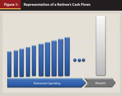
Tension exists between spending and bequest. The more one spends in retirement, the less wealth there will be to bequeath. In an extreme case, if a retiree runs out of money in retirement the bequest amount can effectively be negative. Unfortunately, it’s not uncommon for children to support impoverished parents in their later years if they run out of money.

As retirees consider spending approaches such as using only interest, dividends, and royalties, they should consider how well the adopted spending policy meets their objectives regarding spending and bequeathing assets.

The remainder of this paper provides evidence that a spending approach that spends only interest and dividends—one that allows principal to grow untouched—is a poor approach for most retirees. To demonstrate this, a simple framework that has been used by many authors in analyzing sustainable withdrawal rates is presented.

Analysis Approach

A 30-year planning horizon was used to evaluate the policy of spending only dividends and interest, while leaving principal untouched. Using a 30-year horizon was introduced by Bengen (1994) to evaluate sustainable withdrawal rates. In this framework, the investment portfolio is judged against its ability to fund 30 years of spending. Remaining wealth at the end of 30 years is assumed to be bequeathed. Most retirement horizons will not be precisely 30 years;⁴ however, a 30-year timeframe provides an illustration of what one might expect if they follow a policy of spending only yield.

Historical data from 1953 to 2013 was used to construct this analysis. The S&P 500 was used as a proxy for equity returns, and the 10-year Treasury yield was used as a proxy to construct fixed-income cash flows. Four different 30-year windows were examined: 1953 to 1983, 1963 to 1993, 1973 to 2003, and 1983 to 2013. Each of these historical periods mimics a 30-year retirement when interest rates, dividend yields, inflation, and market returns varied. Figure 2 shows the 10-year Treasury rate over the entire history.

As shown in Figure 2, the past 60 years had windows of rising and falling interest rates. The window covering the 1953 to 1983 period is indicative of a time of rising interest rates, while the period from 1983 to 2013 is indicative of a falling interest rate environment. The two middle windows had both a rising and falling interest rate trends.

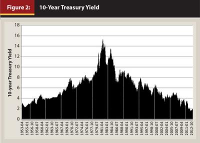
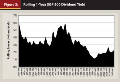
Figure 3 shows that the history of the S&P 500 dividend yield started out fairly high, producing nearly 6 percent in 1954, primarily oscillating until 1982 when it again reached nearly 6 percent, then trended downward until 2000 when it was just above 1 percent. Since 2000, the yield trended modestly upward. The selected 30-year windows cover these oscillatory yield periods.

The inflation rate over the period of analysis was mostly oscillatory except during the latter part of the 1970s and into the early 1980s when inflation surged for several years, reaching nearly 12 percent in the mid-70s, and beyond 14 percent in the late 70s.

Similar to inflation, S&P 500 returns over the period of analysis have exhibited both good and bad returns.

Consistency of Yield Paychecks

A retiree’s monthly expenses are typically stable. Given this, all else being equal, spending policies that produce variable cash flows are likely less desirable than ones that produce consistent cash flows. How consistent are cash flows produced from yield? To answer this question the cash flow consistency coming from fixed income investments held in a 10-year Treasury bond ladder and also from S&P 500 equity dividends was examined.

Figure 4 demonstrates the historical cash flows that a 10-year bond ladder using zero coupon Treasuries would have produced. Each bar represents the interest that would have been earned on a $100 zero coupon Treasury investment 10 years prior. Each month when a bond matures, the initial $100 principal was assumed to be reinvested and the accrued interest was assumed to be spent. It was further assumed that 120 bonds were held in the bond ladder.

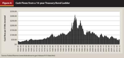
Figure 4 shows that the pattern of cash flows produced by the Treasury bond ladder was quite variable. The pattern does not conform well to a stable, inflation-adjusted retirement spending need. Table 1 confirms this insight by showing cash flow statistics for a bond ladder over three different historical windows.

Table 1 has several notable points. The spending amount generated from the bond ladder is variable and depends on the yield 10 years prior. Because the 10-year Treasury yield is stochastic, there is variability in the cash flows coming from the bond ladder. This variability is similar to stock market volatility. Whether or not the cash flows keep pace with inflation depends on the trend of the yield.

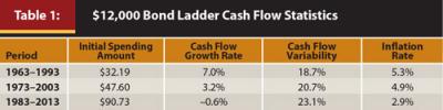
During the first 30-year period when yields rose substantially (1963–1993), the cash flows coming from the bond ladder actually grew faster than inflation, on average. In the second period, which covers both the rise and fall of yields, cash flows grew roughly in line with inflation. However, cash flows were actually rising faster than inflation and then falling relative to inflation. In the final period (1983–2013), cash flows were, on average, flat. In summary, cash flows coming from yield are anything but stable, with trends that are not meaningfully aligned with a consistent inflation-adjusted spending need.

Are cash flows produced from S&P 500 equity dividends any more consistent than the cash flows from bonds? It is possible to use dividends of the S&P 500 Index as a proxy to demonstrate that cash flows coming from dividends change over time. Most investors seeking dividend yield would use a higher dividend yield investment than one indexed to the S&P 500; however, the goal here is to simply show how cash flow levels coming from dividends and the variability of these cash flows have changed over time.

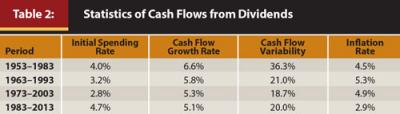
Table 2 shows how cash flows generated from dividends varied over the historical period analyzed. These data produce several notable observations. First, the level of cash flow coming from dividends varied with the period analyzed. For example, the starting cash flow in the 1983–2013 period was nearly twice the starting cash flow compared to the 1973–2003 period. Second, the cash flows coming from dividends over these periods have outpaced inflation. This means that relative to an inflation-adjusted cash flow targets, the cash flows grew at a faster pace. Finally, the cash flow variability⁵ from month to month and year to year was material. For a retiree with bills that do not fluctuate, this kind of volatility in a cash flow stream is likely undesirable.

Yield Paychecks Sub-optimize Spending and Estate Objectives

To examine the level of spending and potential bequest amounts, the following discussion looks at a portfolio of bonds mixed with S&P 500 equities. The portfolio starts with $1 million. Forty percent was assumed to be invested in a bond ladder, with 60 percent invested in the S&P 500. The portfolio was not rebalanced over time. The principal of the bonds maturing in the ladder and the principal of the S&P 500 equity were assumed to remain invested, while interest and dividends would be spent. Figure 5 shows the real spending level over time for three different periods in the history of the initial 60 percent equity/40 percent bond portfolio. (The window starting in 1953 was not used because there is no data to construct a bond ladder starting in 1953.)

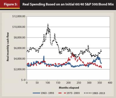
As seen earlier, cash flows coming from this mixed portfolio are still quite volatile. In each historical time period, the maximum real spending level was roughly twice the minimum spending level. Interestingly, the initial real value of spending and final real value of spending over each window of time were not hugely different despite the variability along the path. Also, the amount of spending across each window was different. Although the first two windows are comparable, the initial spending over the 1983 through 2013 period was nearly double the spending level of the other two windows.

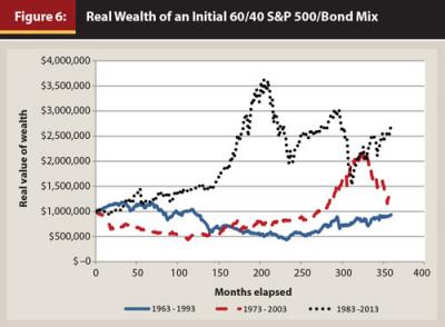
Just as retirees should be concerned about spending levels and variability, they should also be concerned with the pattern of their wealth used to generate the cash flows. Bequeathing a large sum of wealth means that the retiree could have spent more. Figure 6 shows the real value of wealth for sample historical windows of the initial 60 percent equity and 40 percent bond portfolio. Spending only interest and dividends does, on average, preserve the real value of wealth. In the 1983 through 2013 history, significant additional real wealth that could be used for bequest was generated because of lower inflation in this window of time. Not running out of money in retirement is obviously a good outcome, but one must question whether this spending policy sub-optimizes spending and bequest objectives.

Depending on the particular preferences of a retiree regarding the spending level, spending variability, and bequest amount, there may be superior spending strategies. For example, some of the wealth earmarked for bequest could be used to raise the spending level if a retiree prefers higher spending relative to bequest. Similarly, some of the wealth surplus that will be bequeathed could also be used to smooth spending. Given that most retirees rank spending needs ahead of estate goals, under-allocating to spending and over-allocating to estate goals becomes sub-optimal.

Despite the findings thus far, rather than considering drawing down the portfolio, some advisers may consider altering a portfolio’s composition to create enough yield to meet desired spending needs. For example, the adviser could reallocate investment grade bonds to high yield funds and emerging market debt because the latter have a yield premium relative to Treasuries and investment grade fixed income assets. Although this does increase the yield, it has other consequences as well. Increasing yield by investing in riskier debt, distressed properties, or deep value securities increases the risk of the principal generating the yield. This translates to higher volatility in the principal, which increases the variability of the cash flows coming from yield. This increased risk could potentially prove catastrophic for a retiree.

Are Yield Portfolios Inefficient Income Generators?

This section shows (with the supporting appendix below) that using yield to generate retirement income is most likely less efficient than drawing down an efficient frontier portfolio. Tilting a portfolio to produce more yield than what is produced by an efficient frontier portfolio makes the yield portfolio less efficient than the efficient frontier portfolio in all but a few isolated cases.⁶

Consider an example where a portfolio is developed with the highest expected return (yield plus capital appreciation) with a volatility of 10 percent using mean variance optimization. Assume this portfolio has a yield of 2 percent. This portfolio is illustrated by the blue dot in Figure 7. Now consider an additional constraint to make the yield at least 4 percent. Adding this constraint cannot improve the total return in the portfolio optimization; adding constraints to an optimization cannot increase the objective value. Therefore, the return will remain the same or become lower. However, if the constraint is binding (which it will be if the desired yield is higher than the efficient frontier portfolio’s yield) in all but limited cases, the total return will decrease relative to the efficient portfolio.⁷ Therefore, the yield portfolio in Figure 7 becomes the orange dot below the frontier. This clarifies the point that tilting a portfolio to produce more yield lowers its efficiency from a risk and total return perspective. 

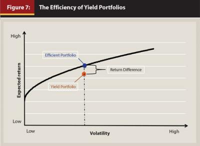
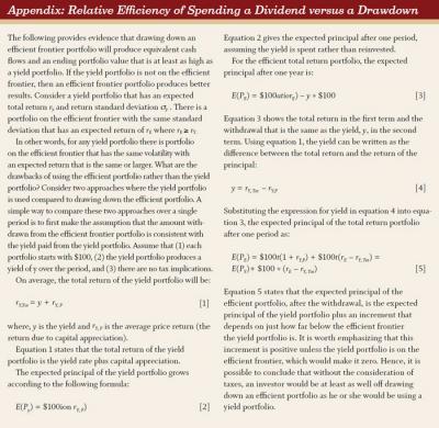
The appendix shows that drawing down an efficient frontier portfolio provides equivalent cash flows to a yield portfolio while also providing higher expected growth of principal; this is true unless the yield portfolio is itself on the efficient frontier. The appendix also shows that if the yield portfolio is on the efficient frontier, before taxes, the efficient frontier portfolio and the yield portfolio produce equivalent cash flows and principal growth. However, if the yield portfolio is not on the efficient frontier, as shown in Figure 7, yield portfolios cannot be better than efficient frontier portfolios at fulfilling spending needs and preserving capital. They are most likely less fulfilling.⁸

Ignoring tax considerations, an investor would be better off drawing down an efficient frontier portfolio than a portfolio that emphasizes yield, when that portfolio falls below the efficient frontier. The effect that taxes have on the efficiency of yield versus capital withdrawals depends on the account type in which investments are held. If the portfolio is held in a tax-exempt account, the conclusion that drawing down an efficient portfolio is superior to investing in a less efficient yield emphasizing portfolio remains unchanged. If the portfolio is held in a tax-deferred account, the analysis in the appendix is also largely unchanged, except that the yield and the withdrawal must be adjusted downward in the same proportion for taxes at the income tax rate. If the portfolio is held in a taxable account, the analysis depends on a few considerations. (Financial advisers should also consider where they locate assets based on the yield of the asset.)

Consider the case of comparing dividend yields to selling shares of equity to meet a cash flow need in a taxable account:

If shares are sold at a loss, there will be no taxes paid when the distribution is made from the efficient drawdown portfolio. Moreover, the losses could be used to offset gains elsewhere. In contrast, a dividend will generate tax according to the investor’s dividend tax rate. 

If shares are sold at a long-term gain, the taxes due on the sale of shares will be less than taxes due from dividends if the dividend and long-term tax rate are the same. Why is this the case? Under current law, taxes are only assessed on capital gains. If an investor sells $100 worth of stock that has a cost basis of $80, the investor only pays tax on the $20 gain. Assuming a 20 percent tax rate, the tax due would be $4. If the investor receives a $100 dividend, under the same assumptions, the tax bill is $20, or five times as much.

If shares are sold at a gain and they have not been held for a year, the comparison of selling shares and dividend distributions depends on the cost basis. The tax from a dividend to meet a $100 cash flow is $20. Suppose the short-term tax rate is 40 percent. If the cost basis of the investment is greater than 50 percent of the value, less tax would be paid using a portfolio withdrawal than using a dividend to meet the cash flow. It’s worth noting that selling a short-term investment that has a cost basis that is 50 percent of the current value means the investment has doubled in value within a year. This is a fairly unlikely, yet fortunate, occurrence. Given the low probability of such high returns, an adviser can easily avoid selling such investments if a diversified portfolio is held.

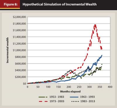
To further substantiate the tax inefficiency of using dividends to fulfill spending rather than drawing down a portfolio, consider the following hypothetical comparisons using S&P 500 historical data. In the first case, the investor spends the after-tax dividends and leaves the principal untouched to grow in the S&P 500. In the second case, assume there is an equity index that perfectly matches the total return of the S&P 500 in every period, but with this investment, no dividends are paid. To fulfill spending needs equivalent to the dividends of the S&P 500, the investor withdrawals an amount from the hypothetical equity investment in the S&P 500.⁹

These two cases illustrate a comparison where after-tax spending and total returns in each period are identical but the tax treatments are different. In one case, the cash flow is taxed as a dividend, and in the other the cash flow is taxed as a long-term capital gain. Of course, there is likely no equity investment that avoids all dividends. However, the point of this comparison is to show that targeting dividends in a taxable account rather than just drawing down the investment is also inefficient from a tax perspective.

Figure 8 illustrates that there is an after-tax benefit associated with paying long-term capital gains tax on withdrawals rather than paying tax on the full dividend distribution. In this hypothetical simulation, on average over the different 30-year windows, the additional wealth generated from deferring taxes by avoiding dividends is $749,778.

In a true application, one cannot likely eliminate all dividends and shift all distributions to long-term capital gains tax treatment. However, many retirees think they should increase their dividend exposure beyond what an efficient portfolio naturally has, however that increases the tax inefficiency. Keep in mind, the current dividend yield is close to 2 percent per year. If a retiree raises the dividend yield of their portfolio for the purpose of generating more cash flows from dividends beyond this to meet cash flow needs, they will experience a tax drag that depends on how much they increase the yield. In taxable accounts, a retiree should actually consider reducing the dividend yield of their investments and instead draw down the portfolio using investment principal and accumulated gains.

From the perspective of meeting spending and growing future principal, investing in an efficient frontier portfolio is superior to investing in a yield emphasizing portfolio (see equation 5 in the appendix). The drawdown can pay the same cash flow and increase the expectation of future principal relative to a yield portfolio. From a tax perspective, if the investor avoids selling short-term gains when the cost basis is less than 50 percent (depending on tax rate) of the investment value, generating cash flows from selling shares is more tax efficient than using dividends to generate cash flows. Other than the behavioral benefit that investors attribute to not selling shares, drawing down an efficient frontier portfolio is a superior way to generate retirement income. Investors who demand the behavioral benefit of not selling shares are paying a high cost for this preference.

Conclusion and Takeaways

Results from this study suggest four important takeaways for financial advisers: First, yields change over time, leading to inconsistent spending for yield-harvesting investors. Second, using a yield portfolio forces an inefficient tradeoff between retirement spending and estate goals. Third, drawing down an efficient portfolio with the same risk as a portfolio emphasizing yield has higher expected principal accumulation, and fourth, drawing down a portfolio is more tax-efficient than using yield to generate retirement income.

Despite the drawbacks associated with a spend-yield-and-preserve-principal-shares approach, the method does provide cash flow while preserving the principal shares of a portfolio. This provides some assurance that a retiree will not die destitute. However, in most cases, this approach significantly sub-optimizes the objectives of a retiree. Retirees should be able to trade off their spending decision, estate funding, and spending plan risk to suit their preferences. Restricting spending to what can be supported by yield does not provide this flexibility. 

To offer retirees a more valuable solution than spending yield and preserving the principal shares of the portfolio, advisers need a framework to sustainably draw down a portfolio. This framework must allow an adviser to allocate a retiree’s portfolio efficiently between spending and estate goals. A planning process and asset allocation strategy can be used to accomplish this. Pittman and Greenshields (2012) and Fullmer (2009) discussed the application of a framework to sustainably draw down a portfolio, meet lifetime retirement spending needs, and achieve estate objectives.

Additionally, there are approaches for setting and even dynamically adjusting withdrawal rates to control the probability of bankruptcy in retirement (see Bengen 1994; Blanchett, Kowara, Chen 2012; Finke, Pfau, Williams 2012; Frank, Mitchell, Blanchett 2011; Guyton 2004; Guyton and Klinger 2006; Kitces 2008; and Pfau 2011). These works provide thoughtful sustainable spending approaches beyond myopically spending yield and preserving principal shares that can improve outcomes for retirees.

Endnotes

1. Prior to retirement (and in retirement) many investors favor stocks that have higher and stable dividend payout ratios. Whether or not higher yielding equity investments offer superior risk-adjusted returns is not the subject of this paper.
2. See Gardner and Fullmer 2008; Bengen 1994; Blanchett 2007; Blanchett et al. 2012; Fan et al. 2013; Finke et al. 2012; Frank et al. 2011; Guyton 2004; Guyton and Klinger 2006; Kitces 2008; and Pfau 2011.
3. Unspent principal is applied to the estate or bequest goal of the investor.
4. A planning approach that considers lifespan uncertainty, such as the one presented by Gardner and Pittman (2013), is a refinement to using 30 years.
5. Cash flow variability was computed as the standard deviation of the percentage change in the monthly cash flow. This value was then annualized by multiplying by the square root of 12. 
6. For background on mean variance optimization and the development of the efficient frontier, see Markowitz (1952, 1959).
7. This result can be deduced by examining a mean variance portfolio optimization problem where the covariance matrix is positive definite. The only way the expected return would not decrease when a binding yield constraint is added is if there is another investment identical to the optimal portfolio but with higher yield. This portfolio would need to have the same expected total return and correlation to all other investments so that it could be a substitute for some lower yield asset in the optimal portfolio. However, this possibility contradicts the assertion of positive definiteness. In this case, the covariance matrix would have to be positive semi-definite.
8. This should not be interpreted to mean that equity portfolios that overweight high dividend securities relative to capitalization weighting are inefficient portfolios. Rather, this means that constraining a portfolio to produce high yield is not a good idea—not even for an investor with income needs.
9. The withdrawal amount was determined so that the investor receives the same amount of cash flow after paying taxes as he or she would have received from the dividend after paying taxes.

References

Bengen, William P. 1994. “Determining Withdrawal Rates Using Historical Data.” Journal of Financial Planning 7 (4): 171–180.

Blanchett, David M. 2007. “Dynamic Allocation Strategies for Distribution Portfolios: Determining the Optimal Distribution Glide Path.” Journal of Financial Planning 20 (12): 68–71.

Blanchett, David M., Maciej Kowara, and Peng Chen. 2012. “Optimal Withdrawal Strategy for Retirement Income Portfolios.” The Retirement Management Journal 2 (3): 7–20.

Fan, Yuan-An, Steve Murray, and Sam Pittman. 2013. “Optimizing Retirement Income: An Adaptive Approach Based on Assets and Liabilities.” Journal of Retirement 1 (1): 124–135.

Finke, Michael, Wade D. Pfau, and Duncan Williams. 2012. “Spending Flexibility and Safe Withdrawal Rates.” Journal of Financial Planning 25 (3) 44–51.

Frank, Larry R., John B. Mitchell, and David M. Blanchett. 2011. “Probability-of-Failure-Based Decision Rules to Manage Sequence Risk in Retirement.” Journal of Financial Planning 24 (11): 44–53. 

Fullmer, Richard K. 2009. “A Framework for Portfolio Decumulation.” The Journal of Investment Consulting 10 (1): 63–71. 

Gardner, Grant. W., and R. K. Fullmer. 2008. “Does Dividend Yield Matter… to the Overall Success of a Retirement Income Portfolio.” Russell Research Report (August).

Gardner, Grant, and Sam Pittman. 2013. “Measuring the Risk of Running Out of Money in Retirement.” Journal of Financial Planning 26 (12): 38–44.

Guyton, Jonathan T. 2004. “Decision Rules and Portfolio Management for Retirees: Is the ‘Safe’ Initial Withdrawal Rate Too Safe?” Journal of Financial Planning 17 (10): 54–67.

Guyton, Jonathan T., and William J. Klinger. 2006. “Decision Rules and Maximum Initial Withdrawal Rates.” Journal of Financial Planning 19 (3): 48–58.

Kitces, Michael. 2008. “Resolving the Paradox: Is the Safe Withdrawal Rate Sometimes Too Safe.” The Kitces Report. May.

Markowitz, Harry M. 1952. “Portfolio Selection.” The Journal of Finance 7 (1): 77–91

Markowitz, Harry M. 1959. Portfolio Selection: Efficient Diversification of Investments. New York: John Wiley & Sons.

Pfau, Wade D. 2011. “Safe Savings Rates: A New Approach to Retirement Planning Over the Lifecycle.” Journal of Financial Planning. 24 (5): 42–50.

Pittman, Sam, and Rod Greenshields. 2012. “Adaptive Investing: A Responsive Approach to Managing Retirement Assets.” Retirement Management Journal 2 (3): 45–54.

Citation

Pittman, Sam. “Is a Portfolio Built to Produce Yield a Sensible Retirement Income Portfolio?” Journal of Financial Planning 27 (8) 52–60.