Standby Reverse Mortgages: A Risk Management Tool for Retirement Distributions

Journal of Financial Planning: August 2012

 

Executive Summary

• Our study considers using an HECM Saver reverse mortgage as a risk management tool in conjunction with a two-bucket investment strategy, coined the standby reverse mortgage strategy (or SRM), in order to increase the probability a client will be able to meet predetermined retirement goals.
• The HECM Saver has unique and attractive features including lower cost; a non-cancellable line of credit; the borrower’s control over when, and if, he or she uses the line of credit; and a line that can be paid back at any time without a penalty.
• The SRM represents an additional source of readily available cash in a bucket strategy to draw upon when clients’ portfolio values deviate substantially from their expected glidepath (where their portfolio should be relative to their capital needs analysis).
• Monte Carlo simulations were performed using real withdrawal rates of 4 percent, 5 percent, and 6 percent; a home value of $250,000; and a portfolio value of $500,000. The SRM strategy was successful through all scenarios.
• We find this risk management strategy improves portfolio survival rates by a significant amount. The improvement in survival rates is attributable to the mitigation of the volatility drain—the risk of having to sell investments when depreciated.

John Salter, Ph.D., CFP^®, AIFA^®, is an assistant professor of personal financial planning at Texas Tech University and wealth manager at Evensky & Katz Wealth Management in Coral Gables, Florida, and Lubbock, Texas.

Shaun Pfeiffer is a Ph.D. candidate in personal financial planning at Texas Tech University, and associate professor in the Department of Business and Economics at Edinboro University in Edinboro, Pennsylvania.

Harold Evensky, CFP^®, AIF^®, is a research professor of personal financial planning at Texas Tech University and the president of Evensky & Katz Wealth Management.

The importance of effective distribution strategies is rapidly increasing as 78 million baby boomers approach retirement over the next decade.¹ The diminished role of defined benefit plans, longer life expectancy, escalating health care costs, and poor equity returns over the last decade are just a few of the issues confronting retirees that create a challenging retirement landscape. Advisers use a mix of distribution strategies and financial products to manage these risks. Costly products, market volatility, and the opportunity cost associated with cash holdings represent a few obstacles with these strategies. Fortunately, an affordable reverse mortgage, the Home Equity Conversion Mortgage (HECM) Saver, was made available in October 2010. This non-cancellable line of credit that borrowers control (hence the reference to “standby”) and that can be paid back at any time without a penalty, may provide a significant risk management solution to practitioners and retirees.

The proposed strategy works by only borrowing from the HECM Saver during bear markets in order to avoid selling assets at depreciated prices, thereby allowing the assets to recover before selling. Specifically, we focus on the line of credit option of the HECM Saver as a substitute for a source of cash. Simultaneous research by Barry Sacks and Stephen Sacks,² recently published in this journal, provides the basic framework of using home equity as a source of cash in times of bear markets. However, our strategy moves a step further by offering a readily implementable alternative
borrowing and payback methodology using the lower cost HECM Saver line-of-credit product within a bucket strategy. Our research uses a simulation model that incorporates projected asset class returns rather than historical returns, correlated returns, and rebalancing of the portfolio. The major contributions of this study are the trigger for borrowing, rebalancing, and paying back the HECM Saver line of credit.

The ultimate goal of this research is to determine whether borrowing from an HECM Saver when market volatility creates an adverse impact on portfolios can increase the probability clients can meet their spending goals. The other implication of this research, rather than just increasing the probability of meeting goals, is increasing the sustainable withdrawal rate for the same probability of success.

Our results suggest that many retirees, and even workers who qualify for the product who are drawing on savings to supplement their earned income, could benefit from the use of an HECM Saver reverse mortgage. Despite growth in demand for reverse mortgages over the last decade, current estimates suggest that less than 2 percent of eligible homeowners elect to use a reverse mortgage in retirement.³ Although reverse mortgages aren’t for everyone, the reluctance to consider use of reverse mortgages in the distribution phase limits the flexibility of distribution strategies; consequently, advisers and retirees have been left with more traditional distribution strategies.

Current Distribution Strategies

The limited role of private annuitization leaves advisers and retirees with sustainable withdrawal strategies based on non-annuitized assets. Reverse dollar-cost averaging, income portfolios, and bucket strategies are the primary approaches to distribution planning. The flaws associated with reverse dollar-cost averaging and income portfolios are noted in the literature,⁴ and have led advisers to adopt different types of bucket strategies.⁵ Investment professionals, in an attempt to avoid excessive costs, taxes, and inappropriate asset allocation, tend to favor bucket strategies over reverse dollar-cost averaging and income portfolios. In short, practitioners are likely to adopt a strategy that retains sufficient short-term liquidity to mitigate the risk of having to dip into the long-term investment portfolio during bear markets.

Cash Flow Reserve Strategy. Some bucket strategies are fairly simple yet effective. Evensky offers a simple two bucket strategy, which is called the cash flow reserve strategy (CFR).⁶ This strategy carves out up to two years of needs from the investment portfolio and places that money in money market and short-term bond investments. The second bucket, or funds that remain after the cash bucket is established, are invested in a total return portfolio in accordance with clients’ investment policy.⁷
The CFR is refilled when rebalancing, when making investment changes, or during a forced sale of the investment portfolio when the CFR bucket is down to two months of living needs. The cash flow reserve strategy has served clients well in the past by reducing volatility drain and transaction costs, and by offering a behavioral benefit of clients’ knowing the source of funds for their short-term needs. However, there is an opportunity cost in setting aside large amounts of cash, and issues with the forced sale if portfolio values are down for an extended period such as during the Great Recession.

Using home equity as a risk management tool in distribution planning may provide retirees with more efficient and effective distribution strategies. As this is a potentially important financial resource that often remains untapped, strategies that incorporate a prudent use of this resource also become important.

Primer on the HECM Saver

Previous reverse mortgage products have been primarily avoided, other than as a last resort, because of cost.⁸ However, the HECM Saver introduced in October 2010 represents a new potential risk management tool for advisers and retirees. The HECM Saver is similar to a traditional HECM Standard reverse mortgage; however, it has substantially lower up-front costs.

The HECM Saver reverse mortgage has some attractive features:

• The borrower controls when, and if, he or she uses the line of credit.
• Loan debt can be paid back at any time without a penalty, or, at the owner’s election, never paid back during their lifetime as long as they remain in their home.
• The income received from the reverse mortgage is tax-free, and the interest, when paid, may be tax-deductible.
• The unused line of credit grows over time, independent of the home’s value, at the same effective interest rate that would accrue to an outstanding loan balance.
• The FHA-insured HECM Saver is a non-recourse loan—upon sale or death, the repayable debt of the mortgage will not exceed the home value. For example, if the loan balance grows to $300,000 and your home value increases moderately over time to $220,000, the client (and potentially the estate) is not liable for any amount owed above the property value upon sale or death. The FHA insurance would reimburse the lender for the amount of the loan above the home value.

The HECM Saver is available for homeowners at least 62 years old and who either own their home or have modest or no mortgage. Any existing mortgage must be paid off or rolled into the reverse mortgage. The ongoing requirements for the mortgage to remain in good standing are that the owner must maintain the home and pay taxes and insurance.

Up-Front Costs. The up-front cost has been significantly reduced relative to the HECM Standard reverse mortgage. The amount of home equity that can be borrowed on the Saver is about 10 percent–18 percent less than for the Standard; however, the up-front mortgage insurance premium decreases from 2 percent to 0.01 percent. Total costs for the HECM Saver include non-interest costs such as an origination fee, closing costs, up-front and ongoing mortgage insurance premiums, and servicing fees, if applicable. The origination fee, which may reduce to zero if the borrower accepts a higher interest rate, is usually 2 percent of home value up to $200,000, and 1 percent above that with a maximum of $6,000. Closing costs are usually $2,000 to $4,000 when accepting a higher interest rate and subsequently lower origination fee. Servicing fees can be up to $35 per month; however, this fee is similar to origination fees in that it is not always imposed on borrowers.

Ongoing Costs. Ongoing interest costs, when and if funds are borrowed, include a variable interest rate and an annual mortgage insurance premium. The variable interest rate is based on the one-month Libor rate (0.2 percent as of August 2011). In addition to the one-month Libor rate lenders tack on an annual margin that is usually between 1.25 percent and 3 percent. Lastly, the Federal Housing Administration (FHA) charges an annual mortgage insurance premium of 1.25 percent. With so many moving parts the following summary of current costs is included to provide better clarity.
A borrower who qualifies today would pay 0.2 percent (the one-month Libor rate), along with a margin of 2.25 percent and the mortgage insurance premium of 1.25 percent, for a total effective interest rate of 3.7 percent. As long as a loan is outstanding, this annual interest rate accrues monthly. The Libor rate adjusts monthly; however, the remaining components are fixed. There may be no origination costs; this will depend on the competitive environment at the time. Closing costs will vary by state. On a home value of $200,000 they would likely be between $2,000 and $4,000. Because the 0.01 percent up-front mortgage insurance premium is minimal, we can assume 1.75 percent of initial home value as a reasonable scenario for up-front costs. Looking at history as a guide, our study concluded that an average one-month Libor rate of roughly 5 percent with a range between 0.2 percent and 11 percent across the life of the loan were reasonable planning assumptions.

Principal Limit Factor. The amount that can be borrowed from an HECM Saver is determined by the principal limit factor (PLF) at the time of loan origination. The PLF represents the percentage of home equity that is available, and can be thought of as a loan-to-value ratio. Currently, the maximum home value is the lesser of the appraised value or the HECM FHA mortgage limit of $625,500, which is the base value to determine the line of credit. The PLF is a function of the age of the youngest borrower and the “expected interest rate.” The expected interest rate is the summation of the 10-year Libor swap rate and the lender’s index margin. In short, the PLF rises with age and diminishes as the effective interest rate increases. Our assumption of a 2.25 percent lender’s margin coupled with setting the age of the borrower at 62 leads to a PLF of 53 percent in today’s interest rate environment. Our results; however, are based on a 33 percent PLF which is roughly the median PLF when using historical 10-year Libor swap rates. The 33 percent PLF is a conservative estimate by today’s standards, but was prudent from the analytical standpoint.

Results are shown for PLF values of 13 percent, 33 percent, and 53 percent, or roughly the historical low, median, and high values had the HECM Saver been around for the history of the 10-year Libor swap rate. Since the introduction of the HECM Saver in 2010, we have seen PLF values at the high end of this range because of the current low interest rate environment. Unusually high swap rates would result in lower PLF values. It is important to note that Libor swap rate data for which these figures are based has a short history and is only available from July 2000 to present.

Why not use a Home Equity Line of Credit (HELOC) in this strategy? When deciding to use a reverse mortgage in this research, we considered two characteristics of the product: non-cancellable and client payback control, critical in providing the flexibility necessary to weather market storms—the downside volatility of the market. Unfortunately we do not know when market storms will occur or how long these storms will last, so we desired flexibility in payback and a guarantee that credit would be available when and if needed. Specifically, HELOC would require some minimum payment be made and there is—as investors experienced during the recession—the very real risk of a HELOC being frozen, reduced, or even cancelled. Additionally, the HELOC credit amount is proportional to home value and does not automatically increase. However, cost of living does increase over time. These are not risks associated with the Saver; the unused line of credit grows independent of home value, the mortgage may not be cancelled or frozen, and there is the flexibility of payback.

There are limitations and disadvantages to the product. First are the minimum age restriction of 62 and the recommendation of little to no mortgage. The reason for the little to no mortgage recommendation is that upon origination, any existing mortgage would have to be rolled into the reverse mortgage or paid off from other resources. In addition, there are costs to set up the reverse mortgage as discussed previously. There is also the stigma of using debt, whether for debt-adverse clients or simply the psychological discomfort of once again creating a debt against the home that may be debt free. Although the bank issuing the mortgage does not own the home, there is a debt established that will need to be paid in the future. Fortunately, balancing conflicting goals is a reality that advisers are well aware of, and as a consequence, we are well versed in educating clients regarding the need to balance their emotional comfort and financial goals.

The Strategy: Combining the CFR and HECM Saver Strategies

Two issues arise with the traditional cash flow reserve bucket strategy. Already noted is the opportunity cost of holding cash. Second, and where the SRM finds its place, is the instance of a bear market in which the cash bucket in the CFR strategy is low or empty, forcing the liquidation of assets at depreciated prices. As believers in mean reversion and that the domestic and world economies will rise over time, we would expect a future appreciation of these assets; however, if we are forced to sell we automatically lock in the loss. In addition to locking in a loss, we have liquidated a portion of assets to fund living, using assets meant for future years. The SRM provides an alternative to refill the cash bucket with no transaction cost, no tax consequences, and possible tax-deductible interest upon repayment. The strategy also allows a reduction in the cash reserve holdings, from as much as 24 months down to 6 months, because of the “standby” source of readily available cash in the reverse mortgage line of credit.

Our proposed strategy combines the CFR two-bucket strategy with an HECM Saver line of credit, essentially creating a three-bucket strategy.

The SRM is only drawn on in the event that a forced sale of assets is needed when the 6-month cash bucket for retirement needs is empty and the portfolio value is “off”—the losses in the portfolio are such that a sale of investment assets is better avoided. The SRM debt is repaid from the investment portfolio when “back”—after market recovery. Otherwise, the traditional CFR strategy is followed.

The biggest question in this research—answered by running many simulations in a lab experiment mode—was which criteria should be used for determining when the portfolio was “off” and “back.” We analyzed various forms of triggers for borrowing and paying back. Trailing 12-month returns were analyzed; however, issues arose with this methodology. First, basing the trigger only on a positive and negative trailing 12-month return poses an issue when the return is down 20 percent, triggering a borrow, but a positive 1 percent return would then trigger a payback, although the portfolio is still down 19.2 percent. On the other hand, take a 20 percent gain in the portfolio, followed by a 1 percent loss. It was not prudent to borrow in this case of a loss because the portfolio is still up 18.8 percent over the two years. Likewise, any simple metric such as a variation of returns (for example, loss of more than 5 percent for “off,” gain of greater than 5 percent for “back”) resulted in the same issue.

Next we analyzed using the previous portfolio value after the last distribution as the payback trigger, using a similar test of whether the value was higher or lower as the borrow and payback trigger. However, this resulted in the same issue we found using returns as the trigger. What needed to be considered was the sequence of returns and their effect on the portfolio over time.
Ultimately, we concluded that from a financial planning perspective, this strategy should be designed to maximize the probability of our clients’ ability to meet their goals, not to maximize gains or maximize the sustainable withdrawal rate. This conclusion led us to develop our use (“off”) and payback (“back”) triggers based on our client’s projected portfolio glidepath value, determined by a classic capital needs analysis. Figure 1 represents an example of a client’s glidepath who has a $500,000 portfolio today and desires a 5 percent real withdrawal rate ($25,000 first year, subsequent years increased by inflation). The portfolio value line is the theoretical glidepath we would expect our clients’ portfolio to follow in order to meet their goals.

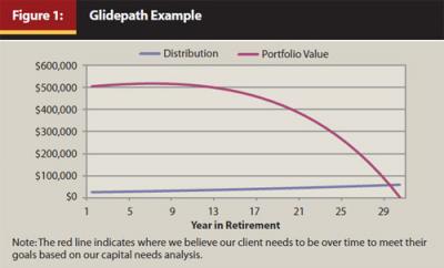
The capital needs analyses we complete for our clients give us this information, and our annual updates allow the glidepath to be fluid and change as the economy and our clients’ needs change. Consequently, the triggers to borrow and pay back the line of credit are adjusted, as necessary, to stay on track with the glidepath: borrowing when below, paying back when above.⁹ However, this research does not include any fluid planning updates. The glidepath is fixed from the onset of the simulation.

Methodology and Strategies

In our study, we use Monte Carlo¹⁰ simulations to test the efficacy of this strategy in retirement planning. First, we simulate 1,000 scenarios. Each scenario represents a hypothetical economic environment (with different interest rates and investment returns for each scenario) for an individual beginning at age 62¹¹ and ending at age 97. Therefore, each simulation has up to 468 months’, or 39 years’, worth of information on interest rates and investment returns. At the beginning of each month, income needs are met using the CFR or, if necessary, drawing from the investment portfolio or using the SRM. The cash reserves, if depleted, are refilled at the end of the month. Similarly, the outstanding loan balance on the SRM is paid down at the end of the month when the portfolio value is above the glidepath mark (defined below). The investment portfolio for all of the strategies is a 60 percent stock/40 percent bond portfolio that is rebalanced back to this initial asset allocation when the stock/bond balance is more than 5 percent out of balance. Assumptions for returns, interest rates, costs, and other important elements of the distribution strategies are included in the appendix.

To summarize the methodology of the SRM strategy in our analysis, an HECM Saver reverse mortgage is used in conjunction with a cash flow reserve two-bucket distribution strategy, ultimately creating a three-bucket distribution strategy. The investment portfolio is used to refill the short-term living expense needs when the portfolio value is above the glidepath in a forced sale (no funds remaining in the CFR) or when rebalancing. In actual implementation, the CFR bucket would also be refilled when making any investment changes, but in our two-asset simulation there are no investment changes other than rebalancing. The reverse mortgage is available when a forced sale is needed but the portfolio is below the glidepath mark.

In other words:

When the portfolio is above the glidepath mark:

• Refill the CFR bucket when rebalancing or making investment changes
• If the CFR bucket is empty, force-sell investment portfolio to refill CFR bucket
• Pay off any loan balance¹² then refill the CFR if needed

When the portfolio is below the glidepath mark:

• If the CFR bucket is sufficient, only rebalance or make investment changes; no refill of the CFR bucket
• If CFR bucket is empty, borrow from reverse mortgage line of credit

Glidepath Mark

After substantial analysis and thought about the glidepath mark, it was determined that using 80 percent of the portfolio value was optimal, both in terms of success and use of the line of credit. Translating this to our previous glidepath figure, our client with $500,000 today using our projected returns would be expected to have $508,686 at the end of this year (after the initial distribution and returns). Twelve months from now if we need to make a decision on a forced sale, our portfolio value marker would be 80 percent of the expected value, or $406,948. If below this value, the refill would be borrowed from the reverse mortgage. If above, a forced sale would be implemented to refill the CFR bucket. Using 100 percent or 90 percent of the glidepath mark resulted in a suboptimal “overuse” of the line of credit, which decreased the success of the strategy in most cases.

Analysis Results

The following are the results of the analysis for one specific client analyzed. Our client is 62 years old, has a portfolio value of $500,000 today and a home worth $250,000. Our client’s spending needs are 5 percent of their initial portfolio, adjusted by inflation each year moving forward. The initial principal limit factor (PLF) for our client is 33 percent, resulting in an available line of credit of $82,500 for the $250,000 home. (As a comparison, today’s environment would result in a PLF of approximately 53 percent, for a line of credit of $132,000.)

Portfolio Survival. As seen in Figure 2, there are significant survival advantages to the SRM strategies. The “6-Month CFR” plot represents the number of portfolios with a positive value at the end of each year denoted in the plot. The “6-Month CFR with Standby RM While IP (Investment Portfolio) Alive” represents the number of portfolios with a positive value when implementing the SRM strategy of borrowing when the portfolio is under the 80 percent glidepath mark. In this alternative, there is no borrowing from the reverse mortgage once the portfolio is exhausted. Once the portfolio is exhausted, the simulation is counted as an unsuccessful scenario. The “6-Month CFR with Standby RM” is identical to the previous alternative, but with as many additional years of income borrowed from the reverse mortgage as possible. In other words, once the portfolio has been exhausted, living needs are borrowed from the reverse mortgage until the line of credit is also exhausted. The reason for separating the latter two analyses was to determine the benefit of the standby strategy itself.

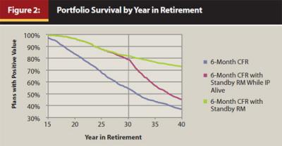
At the 30-year mark of retirement, or when our client is 92, we see the probability of their portfolio having a positive value is approximately 52 percent. When we implement the SRM strategy we find the probability dramatically increases to 78 percent. When the line of credit is used to fund living after the portfolio is exhausted, the probability increases to 82 percent.
It is important to note that our projected returns, as opposed to historical returns, include a lower long-term return on assets than historical, but similar volatility. This results in the stand alone CFR strategy exhausting portfolios more often than it would have historically; however, there is significant academic and practitioner support for the belief that this more stressful economic environment is the future our clients will be facing. As a benchmark, using historical returns, the probability of success of the CFR strategy was approximately 75 percent after 30 years, compared to 52 percent with projected returns.

Also note, though not pictured for clarity, Monte Carlo analyses often are shown with “tornado” or “spaghetti” plots, where a random sample of the trials is plotted. In this analysis, there are, of course, plans that prematurely exhaust the portfolio. What was not taken into account in this analysis is that proper planning would not be based on “invest and forget.” Rather, planning would be regularly updated and adjusted for past and anticipated future markets. In these cases, a recommendation to decrease spending because the portfolio would be on a path to premature exhaustion would be prudent. This would result in a new—and most likely lower—glidepath for those failing plans.

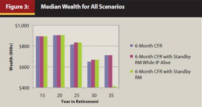
Median Wealth. Median future wealth throughout retirement was calculated and is reported in Figure 3. Note that for the CFR/Standby strategy, median wealth is not sacrificed until later years—for this case after 30 years. The median wealth diminishes for the overall strategy at year 35 because of more than half of the plans not having a positive portfolio value, and many using the full line of credit to fund those few more years of living needs. Note in year 35, the CFR and CFR with Standby While IP Alive have a higher value compared to the full CFR with Standby strategy. This difference represents the untapped value of the home, further suggesting the importance of using this financial resource.

Details on Use of the Strategy

In addition to analyzing the benefits of the SRM strategy, we also analyzed the strategy’s use after 39 years. As noted before, clients (and planners) may have issues with the use of mortgage debt. Surprisingly, the use of the line of credit is not as prevalent as may be expected for portfolios that are successful at meeting clients’ spending needs over the full period. Keep in mind there are simulations in which the sequence of returns resulted in a portfolio trajectory toward premature exhaustion that even this strategy couldn’t prevent—trajectories for which the only recourse would have been decreased spending. These failing plans are more likely to have used the line of credit, carrying a balance for a prolonged period in recession-like markets, as well as used the line of credit to fund a few more years’ needs. In practical terms, planners would carefully monitor and revise plans based on overall portfolio performance and spending pattern, altering the projected glidepath. Because of this, the following analytics focus on simulations up until the portfolio was exhausted.The following does not include use of the reverse mortgage for funding income needs after the portfolio is exhausted.

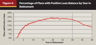
Plans with a Positive Loan Balance. As seen in Figure 4, for our client, the percentage of plans over the 40-year period with a positive loan balance was approximately 24 percent, meaning, at maximum, only one-quarter of all future 1,000 scenarios had a line of credit balance at any given point.

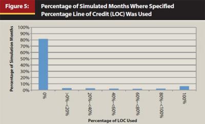
Percentage of Line of Credit Used. The next use attribute analyzed was the percent of the successful simulated months in which a specified percentage of the line of credit was used. As shown in Figure 5, the vast majority of months (approximately 82 percent) had no balance in the line of credit. At the other extreme, only approximately 6 percent of all simulated months resulted in the line of credit being tapped out, or 100 percent used. Thus, even for those clients hyper-sensitive to the issue of using credit, the likelihood of establishing any permanent debt is extremely small and only likely to occur under extremely negative economic conditions. As noted earlier, this is a risk management strategy, not a debt leverage strategy.

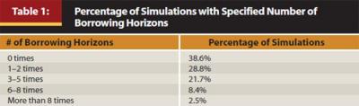
Borrowing Horizons and Frequency. The borrowing horizon was defined as the time between an initial borrow and a full payback. As an example, if money were borrowed today, and again six months from now, but paid back 18 months from now, this would be classified as one borrowing horizon. Note there were two individual borrows from the line of credit for this one borrowing horizon example.

Table 1 shows that borrowing horizons for successful plans ranged from “none,” accounting for approximately 39 percent of simulations, to more than eight, accounting for less than 2.5 percent of all simulations.

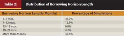
The length of each borrowing horizon per simulation was analyzed and resulted in an interesting finding. In the previous example, the borrowing horizon lasted 18 months. As seen in Table 2, the longest length of over 24 months occurs at approximately the same frequency as 1–6 months. Upon further inspection, we found a positive relationship between the probability of the portfolio lasting and borrowing time horizon, meaning longer borrowing horizons were associated with a higher probability of the portfolio having assets to fund goals. However, some of the very long borrowing horizons were associated with failing plans that never recovered to above the glidepath mark.
 

The actual number of borrows was also analyzed. Simulations with 1–20 total borrows occurred in approximately 24 percent of all simulations, 21–40 total borrows occurred in approximately 10 percent, and more than 40 borrows occurred in approximately 8 percent of simulations.

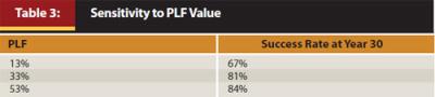
Sensitivity to PLF Factor. As can be expected, the results are positively associated with the actual line of credit that can be obtained based on the: (1) PLF factor (which calculates the loan to value) and (2) the proportion of home value to portfolio size. The larger the line of credit to the portfolio size, the more beneficial the strategy in terms of success defined as a positive portfolio value at the end of a specific period. Because PLF is based on the Libor swap rate, we found, based on historical Libor swap rates, our 62-year-old client could have obtained a PLF factor of between 13 percent and 53 percent at any time in Libor swap history, with a median of 33 percent. Table 3 offers the difference in success after 30 years based on these three possible PLF factors at the onset age of 62. Table 3 success rates are in relation to the same 52 percent success rate after 30 years for the CFR strategy.

Sensitivity to Libor and Returns. We also analyzed the sensitivity to Libor rates, resulting in the cost of borrowing, and portfolio returns. Results suggest, in terms of simple success in the portfolio (having assets after a certain period) or premature portfolio exhaustion, that returns contribute much more to success or failure than Libor rates. However, when looking at the top decile (best 10 percent) in terms of ending portfolio value versus the bottom decile (worst 10 percent), both Libor rates and portfolio rate of return contributed to being in either decile. But in terms of a simulation having assets to fund goals or not, there was little difference in Libor rates of the plans that succeeded or failed.

Additionally, we analyzed 11 other combinations of withdrawal rates, portfolio values, and home values. Across all combinations, we found similar results in terms of the strategy increasing the probability that clients could meet their goals. Although there were slight variations in the metrics of use, no major deviations were noted. However, there was a positive relationship between use and the withdrawal rate, as would be expected.

Conclusions

The main conclusion of this study is that HECM Saver reverse mortgages do have a place in mainstream retirement distribution planning, and have a significant impact on the probability that some clients will be able to meet their predetermined retirement goals. Updating plans during prolonged bear markets or severe market drops, along with this strategy, has the possibility of further increasing this chance of success.

As the principal limit factor provides the loan-to-value ratio of the line of credit, it is a significant element in determining success. The higher the PLF, resulting in a higher line of credit, the higher the success rates. Similarly, the larger home value relative to portfolio size results in an increased success rate resulting from the larger line of credit relative to portfolio size, due to an increased relative borrowing capacity.

In terms of success or premature exhaustion of the portfolio, returns have a much higher impact than Libor rates. However, extremely high Libor rates do become quite significant. Libor swap rates influence the PLF factor. At times of high Libor swap rates, the PLF factor is reduced, thereby reducing the ultimate line of credit amount. Consequently, investors should use caution in setting up an HECM Saver line of credit in these times. In addition, subject to the friction of refinance costs, HECM Saver reverse mortgages can be refinanced at a later date to take advantage of more advantageous conditions.

The study suggests that if long-term rates of return are well below historical rates, but maintain similar volatility, the SRM strategy may be much more valuable.

The SRM strategy is appealing for four primary reasons: it diminishes the size of the cash bucket and consequently the opportunity cost of holding cash; it provides flexibility in that the investment bucket is not sold during bear markets; it allows the retiree to decide how much home equity is used to meet needs if the investment bucket is exhausted; and most importantly, it increases the life expectancy of an investor’s nest egg.

Endnotes

1. U.S. Census Bureau. 2010. Age and Sex Composition: 2001. Retrieved September 2, 2011, from www.census.gov/prod/cen2010/briefs/c2010br-03.pdf.
2. Sacks, B., and S. Sacks. 2012. “Reversing the Conventional Wisdom: Using Home Equity to Supplement Retirement Income.” Journal of Financial Planning (February).
3. The National Retirement Risk Index Fact Sheet No. 1. 2010. “The NRRI and the House.” Center for Retirment Research at Boston College (March). http://crr.bc.edu/special-projects/nrri/fact-sheet-the-nrri-and-the-house/.
4. Otar, J. 2002. “Live Long and Prosper!” Financial Planning (July): 67–70.
5. Evensky, H. 2006. “From Accumulation to Distribution.” Financial Planning (May): 70–75.
6. Evensky, H., T. Robinson, and S. Horan. 2011. The New Wealth Management. Hoboken, New Jersey: John Wiley & Sons Inc.; Evensky, H., and D. Katz, eds. 2006. Retirement Income Redesigned. New York: Bloomberg Press.
7. This is the assumed allocation in our study; however, the retiree should consult a financial planner to determine the appropriate mix of investments.
8. Davidoff, T., and G. Welke. 2004. “Selection and Moral Hazard in the Reverse Mortgage Market.” Working paper.
9. As the strategy is designed to achieve our client’s goals, not maximize portfolio value, if above the glidepath and in a forced-sale circumstance, the investment portfolio is liquidated to fill the bucket.
10. Rolling 30-year period analysis using historical data from 1926 is available from the authors at request. Results of the strategy were similar to projected returns in this analysis.
11. Each analysis begins at age 62, which is the date of first qualification for a reverse mortgage.
12. Note that a very modest minimum balance needs to be held to keep the line of credit in good standing. A de minims trade rule was modeled requiring a minimum line of credit balance of $3,000 as to not incur a transaction charge to pay off a relatively small balance.

Appendix: Assumptions

• Portfolio Allocation, Transaction Costs, and Rebalancing. The initial asset allocation on the portfolio is 60 percent equity/40 percent bond and is rebalanced back to the initial allocation when one of the asset classes deviates by 5 percent (absolute) or more from the initial percentage. Transaction costs are assumed to be $30. Our simulations do not take taxes into account; we assume a non-tax environment, meaning distributions are gross of taxes.
• Initial Asset Class Values and Returns. Broadly speaking, there are four main asset classes: the home, stocks, bonds, and cash. The initial home value analyzed is $250,000, and appreciates monthly at a constant annual nominal rate of 3 percent. The investment portfolio value was modeled at $500,000. Stock and bond returns follow a lognormal distribution. The mean projected annual nominal return is 8.7 percent (23 percent standard deviation) and 5.4 percent (6.1 percent standard deviation) for stocks and bonds, respectively. The mean annual nominal return on cash is 3 percent.
  
  As to questions about what happens if a home depreciates in value, the HECM Saver line of credit increases relative to the Libor rate, not the home value rate. There is no point in varying the home value once the reverse mortgage is taken out; the line of credit value will not change with the home value. The loan is non-recourse, meaning the owner will not owe more than the home is worth if there is a debt.
• Interest Rates and Inflation. The one-month Libor rate, lender’s margin, mortgage insurance premium, and 10-year Libor swap are the four interest rates that are important in the simulations. Interest accrues and adjusts on a monthly basis. The mean one-month Libor rate is modeled at 5 percent and has a range of 0.2 percent to 12.5 percent. We assume a constant 2.25 percent for the lender’s margin, which leads to an assumption of no origination fee. The 10-year Libor swap mean annual rate is assumed to be 4.7 percent. The 10-year Libor swap rate does not affect borrowing costs; however, it plays a key role in how much equity can be accessed from the home. The annual mortgage insurance premium is a constant 1.25 percent, which is equivalent to the current FHA standards. Inflation is assumed to be constant at an annual nominal 3 percent rate.
• Non-Interest Costs. Non-interest costs include origination costs, closing costs, monthly service fees, and the up-front mortgage insurance premium. We assume no origination costs because of our assumption of a higher margin (2.25 percent). A closing cost estimate was assumed to be a very conservative 1.75 percent of the home value. No monthly service fee is assumed, and the up-front mortgage insurance premium is 0.01 percent of home value. All costs are financed by the reverse mortgage rather than being paid from assets at time of establishment.