Journal of Financial Planning: August 2011
Executive Summary
- This paper investigates how well market valuation and yield measures predict the maximum sustainable withdrawal rate (MWR) people can use with their retirement savings to obtain inflation-adjusted income over a 30-year period.
- The regression framework includes variables to predict long-term stock returns, bond returns, and inflation (the components driving a retiree’s remaining portfolio balance). It produces estimates that fit the historical data well.
- This study suggests that, in projecting long-term sustainability for recent U.S. retirees, a 4 percent withdrawal rate cannot be considered safe when the cyclically adjusted price-earnings ratio has experienced historical highs and the dividend yield has experienced historical lows.
- Nevertheless, there are important qualifications for these predictions. Most importantly, they depend on out-of-sample estimates, as the circumstances of the past 15 years have not been witnessed before.
- Readers persuaded by this analysis may wish to include TIPS and other assets in their portfolios, and recent retirees should closely monitor their spending and portfolio balances. Maintaining flexibility with retirement spending is important.
- More generally, this framework can guide new retirees toward a reasonable range for their expected MWR so that the 4 percent rule need not be blindly followed.
Wade D. Pfau, Ph.D., an associate professor at the National Graduate Institute for Policy Studies in Tokyo, Japan, holds a doctorate in economics from Princeton University. His hometown is Des Moines, Iowa. He can be reached at wpfau@grips.ac.jp.
Acknowledgments: I am grateful for the insightful comments from this journal’s anonymous reviewers, for a variety of related discussions provided at the Bogleheads Forum, and for financial support from the Japan Society for the Promotion of Science Grants-in-Aid for Young Scientists (B) # 23730272.
Consider two hypothetical individuals. Each saved 10 percent of her salary at the end of each year over the final 30 years of her career for the purpose of helping to fund her retirement. Each experienced salary growth that matched the inflation rate. Each invested her growing portfolio of wealth in a 60/40 asset allocation of stocks and bonds, rebalanced at the end of each year. The difference: one of these individuals retired in 1921, and the other retired in 2000. Figure 1 shows the wealth accumulation path for each retiree during the 30-year accumulation phase.
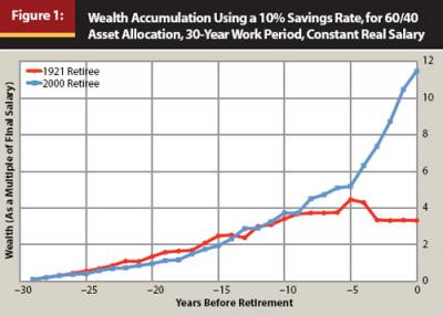
Despite having the same salary pattern and the same fixed 10 percent savings rate, the 2000 retiree entered retirement with wealth totaling 11.48 multiples of her final salary, and the 1921 retiree’s portfolio held only 3.32 times her final salary. Nevertheless, this divergent outcome could hardly have been guessed earlier. It was only in the final five years of their respective careers that their experiences remarkably diverged, and the 1921 retiree even enjoyed a larger portfolio balance during most of the first 18 years of their respective careers.
We are rather dependent on what happens in financial markets during our final work years (this dependency is also known as the “portfolio size effect” because a given percent change in portfolio value has a larger absolute impact when the portfolio is bigger; Bernard (2011) provides Michael Kitces’s thoughts about this matter). These two hypothetical retirees were chosen because, with the historical data since 1871 used in this study, they are the retirees who experienced the largest and smallest wealth accumulations of anyone using a fixed savings rate over 30 years.
Traditional Retirement Planning Approach
Traditional retirement planning advice involves deciding well before retirement on a withdrawal rate that can be reasonably viewed as safe, and then trying to accumulate enough wealth by retirement so that the withdrawal amount from one’s wealth using one’s chosen withdrawal rate matches one’s desired retirement expenditures. For a retirement portfolio split between stocks and bonds, the maximum sustainable withdrawal rate (MWR) over a 30-year horizon is the initial withdrawal amount as a percentage of wealth accumulation at retirement that can then be adjusted for inflation in subsequent years and will provide income for precisely 30 years. Determining a safe withdrawal rate has been an active goal of researchers since the seminal Journal of Financial Planning article by Bengen (1994), which originated a methodology for finding a safe real withdrawal rate using historical data. His SAFEMAX is the minimum of all the MWRs in the historical period.
As reported by Bengen (2006), this value was about 4.1 percent for stock allocations between 37 percent and 67 percent. MWRs vary from study to study because they are quite sensitive to underlying assumptions about asset allocation, data sources for asset returns, whether any fees are deducted, whether analysis is made on a monthly or annual basis, whether withdrawals occur at the beginning or end of each period, and how frequently the portfolio is rebalanced. Bengen (2006) updated his earlier work to incorporate small-capitalization stocks along with the S&P 500 and intermediate-term government bonds, and he found that the SAFEMAX increases to about 4.5 percent.
By 2011, countless current and prospective retirees have relied on the tables of success rates provided by the Trinity study, which was recently updated in the April 2011 Journal of Financial Planning by Cooley, Hubbard, and Walz (2011). They show, using rolling periods from the historical data, the success rate for various fixed and inflation-adjusted withdrawal rates using various asset allocations and for various assumed retirement lengths. Though results vary by expenditure strategies, asset allocation, and allowances for potential failure, the basic idea for this study’s users can be provided with an example. A retiree plans for 30 years of inflation-adjusted withdrawals and decides on a 50/50 strategic asset allocation of stocks and bonds in retirement. Using the study’s Table 2, the retiree learns that a 4 percent withdrawal rate worked in 96 percent of the 30-year rolling periods from the historical data. If our previously mentioned retiree decided this was a reasonable success rate and settled on using 4 percent for her withdrawal rate (assuming, of course, that her desired retirement spending needs were not less than 4 percent), the 1921 retiree would only obtain a withdrawal amount equal to 28.9 percent of the withdrawal amount enjoyed by the 2000 retiree, who had accumulated 3.46 times as much wealth.
An Alternative Perspective
Should both the 1921 retiree and the 2000 retiree follow the traditional advice exemplified here by using a 4 percent withdrawal rate? In the May 2011 Journal of Financial Planning, Pfau (2011a) suggests that the answer is no. Rather, by linking the accumulation and retirement phases together, it becomes clear that “the lowest sustainable withdrawal rates (which give us our idea of the safe withdrawal rate) tend to follow prolonged bull markets, while the highest sustainable withdrawal rates tend to follow prolonged bear markets.” That article suggests, instead, that retirement planning should focus on the savings rate needed to finance one’s desired retirement expenditures regardless of the actual withdrawal rates required under the framework. But focusing on savings rates is of little value to those already on the cusp of retirement. The present study fills the gap by extending the underlying framework in Pfau (2011a) regarding the effects of bull and bear markets to consider whether new retirees may be able to predict their sustainable withdrawal rate given the market conditions facing them at their retirement date.
Indeed, the smallest and largest wealth accumulations are not the only records set by the retirees in 1921 and 2000. In January 1921, the cyclically adjusted price-earnings ratio (PE10), defined as the stock index price divided by the average real earnings from the previous 10 years, was 5.12. This was the lowest value of any January in the historical period. Meanwhile, PE10 in January 2000 was 43.77, the highest in history. These extremes compare to a 16.43 historical average. In addition, the 1921 retiree with a 60/40 asset allocation experienced another important record, as this retiree enjoyed the highest maximum sustainable withdrawal rate in history (10.42 percent). Will the 2000 retiree therefore experience the lowest maximum sustainable withdrawal rate in history? This will only be known after data through 2029 is available, but exploring this possibility is the topic of the present study.
The basis for this approach is Campbell and Shiller’s (1998) finding that earnings valuation ratios provide predictive power for long-term stock market returns. Most notably, the dividend-price ratio or dividend yield (DY) and the ratio of current stock price to average real earnings over the previous 10 years (PE10) are both predictors of the subsequent 10-year real returns on stocks. Whether this relationship can be treated as statistically significant has plagued researchers since Campbell and Shiller’s initial work. Estimating correct standard errors and statistical significance is confounded by the problems of overlapping observations and serial correlation created by the use of rolling historical periods. In reviewing the debate, Shiller (2006) focused on the economic significance of the relationship rather than the formal statistical significance, stating, “A regression would not indicate a terribly good fit, but it is a good enough fit to suggest that there is something to this model.”
The approach taken by a number of earlier withdrawal rate studies does not properly emphasize what we can learn from the historical data. Writing more generally about forecasts for future stock returns, Bogle (2009, p. 102) said, “My concern is that too many of us make the implicit assumption that stock market history repeats itself when we know, deep down, that the only valid prism through which to view the market’s future is the one that takes into account not history, but the sources of stock returns.” These sources include income, growth, and changing valuation multiples. For stocks, returns depend on their dividend yield, earnings growth, and any changes in the valuation placed on earnings. If the current dividend yield is below its historical average, then future stock returns will also tend to be lower. In contrast, when the PE10 is low, markets tend to exhibit mean reversion, and relatively higher future returns can be expected. Returns on bonds depend on the initial bond yield and on subsequent yield changes. Low bond yields tend to translate into lower returns because of less income and heightened interest-rate risk. Sustainable withdrawal rates are intricately related to the returns provided by the underlying investment portfolio. The historical average success rate for a withdrawal strategy is not the information retirees need to know when determining their forward-looking sustainable withdrawal rate.
An important point about the historical data must be made clear. It is natural to think that withdrawal rate studies based on historical data will have accounted for the full range of observed valuation levels, and that the 4 percent rule has withstood the test of time. This is correct only to an extent. If one is using asset returns data through the end of 2009, then 30-year MWRs can be calculated for retirements beginning only up to 1980. As Cooley, Hubbard, and Walz (2003) suggest, this means recent years count for less as they show up in fewer rolling historical periods. But more importantly, Pfau (2010) demonstrates that retirement success is more dependent on what happens early in retirement than late in retirement. In fact, the wealth remaining 10 years after retirement combined with the cumulative inflation during those 10 years can explain 80 percent of the variation in a retiree’s 30-year MWR. Altogether, events that took place since about 1990 contributed little to the portfolio success rates in studies such as Cooley, Hubbard, and Walz (2011).
Although debates about whether market fundamentals should be incorporated into withdrawal rate studies have raged on Internet discussion boards related to personal finance since as early as 2002, financial practitioners may have been made most aware of the issue by Kitces (2008a). He investigated the relationship between safe withdrawal rates and PE10. He divided the historical PE10 values into quintiles and then showed the lowest and highest MWRs within each quintile. He concluded that retirees should be cautious when retiring at times with high PE10 ratios, but he still expected a 4.5 percent withdrawal rate to be safe. His focus was more in the other direction—retirees who observe a PE10 value below 12 at retirement could safely increase their withdrawal rate to 5.5 percent. In a subsequent blog post on the matter, though, Kitces (2008b) amended his previous conclusion to note that the previously unseen high valuation levels of the late 1990s and early 2000s could potentially lead to new lows for MWRs in those years.
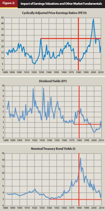
Figure 2 illustrates why recent retirees may be concerned about the impact of earnings valuations and other market fundamentals on their retirements, as the situation for market fundamentals since the mid-1990s (the period that barely affects the results of earlier studies, as mentioned above) is remarkably different from that experienced in earlier historical periods. For PE10, the highest value in a January before 1980 was 27.08, which happened in 1929. Since 1980, though, PE10 was above 27.08 in eight different years, including 1997–2002, 2004, and 2007. A high point of 43.77 occurred in January 2000. Meanwhile, for the pre-1980 period, the dividend yield reached a historic low of 2.67 percent in January 1973. But in every year since 1996 (except 2009), the dividend yield has fallen below this value. The possibility exists that companies replaced dividend payments with stock buybacks that increase earnings per share, but Campbell and Shiller (1998) and Rob Arnott (cited in Arends 2010) do not find this explanation sufficient to eliminate worries about lower dividend yields. Additionally, the nominal 10-year bond yield reached a historic low of 1.95 percent in January 1941, and though recent levels are not near historic lows, they are also not particularly high and cannot help much to counteract the other factors that may tend to depress sustainable withdrawal rates.
This study attempts to predict sustainable withdrawal rates by quantifying whether a 4 percent withdrawal rate can still be considered safe for U.S. retirees in recent years when stock market valuations have been at historical highs and dividend yields have been at historical lows. I find that a regression model using market fundamentals can explain historical MWRs fairly well, and that the 4 percent rule is likely to fail for recent retirees. Despite the peak for PE10 in 2000, I find that MWRs may continue to decline after 2000 as the continued falling dividend yields and bond yields offset falling earnings-valuation levels. There are important qualifications for these predictions discussed in the conclusion. But generally, this study complements my argument in Pfau (2011a) that “worrying about the ‘safe withdrawal rate’ and a ‘wealth accumulation target’ is distracting and potentially harmful for those engaged in the retirement planning process” by providing a methodology to guide new retirees toward a reasonable range for their sustainable withdrawal rate. The 4 percent rule need not be blindly followed regardless of present economic circumstances.
Methodology and Data
The maximum sustainable withdrawal rate (MWR) is the variable I seek to explain and predict. For each retirement year, it is the highest withdrawal rate that would have provided a sustained real income over the subsequent 30-year period. At the beginning of the first year of retirement, an initial withdrawal is made equal to the MWR multiplied by accumulated wealth. Remaining assets then grow or shrink according to the asset returns for the year. At the end of the year, the remaining portfolio wealth is rebalanced to the targeted asset allocation. In subsequent years, the withdrawal amount adjusts by the previous year’s inflation rate, and the order of portfolio transactions is repeated. Withdrawals are made at the start of each year and are not affected by asset returns, so the current withdrawal rate (the withdrawal amount divided by remaining wealth) differs from the MWR in subsequent years. If the withdrawal pushes the account balance to zero, the withdrawal rate was too high and the portfolio failed.
No attempt is made to consider taxes, which makes these findings applicable to Roth IRAs when considered on an after-tax basis. (Bengen [2006] did analyze the impacts of taxes on withdrawal rates.) Also, for these results, I assume that retirees do not need to pay any portfolio management or adviser fees. However, Pfau (2011b) provides more details about the impact of fees for the data used in this study. With a 60/40 asset allocation, a 1 percent account fee charged at the end of each year would, on average, result in a 0.63 percentage point reduction in the MWR, which represents an average reduction in retiree annual spending power of 11 percent (compared with the MWR) from her wealth portfolio.
Data are from Robert Shiller’s website (www.econ.yale.edu/~shiller/data.htm). The data include large-capitalization stock index values and total returns, 10-year government bond yields and total returns, the consumer price index, aggregate dividends, and aggregate corporate earnings since 1871.
I develop a regression model to predict the 30-year MWR for a retiree based on market information freely available at the start of retirement. I choose one regression specification to cover the various asset allocations, which suggests that the specification must include variables to predict real stock and bond returns and inflation. Campbell and Shiller established a link between real stock returns, PE10, and DY, suggesting that these variables belong in the model. PE10 is the stock price in January divided by the average real earnings on a monthly basis over the previous 10 years. Campbell and Shiller justified this measure as a way to remove cyclical factors from earnings, though there is no particular theoretical reason to choose precisely 10 years. The cyclically adjusted earnings yield (EY10) is 100 divided by PE10. I use EY10 rather than PE10 for the main predictions and forecasting, as the out-of-sample predictions of MWRs from simple one-variable regressions show that the EY10 regression is more forgiving of low EY10 values than the PE10 regression is of corresponding high PE10 values. PE10 predicts worse MWR outcomes in recent years, but is more vulnerable to out-of-sample estimation errors. For this reason, predictions for recent MWRs should rely more on EY10 than PE10.
The dividend yield (DY) is aggregate dividends divided by the stock price. I find that a 10-year moving average for the dividend yield (DY10) provides a better model fit. This can be justified as a way to obtain the underlying trend in dividend payments after removing the cyclical trend in stock prices. Unlike EY10, the 10-year moving average for DY is not the average of previous dividends over current price, but rather the average dividend yield. Because EY10 already includes the current price, another variable with current price is not needed.
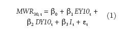
Nominal bond yields (I) are for 10-year government bonds. For bond returns, this yield may provide reasonable predictive power, as a high yield implies both that current income from the bond will be high and that any subsequent shift toward lower yields will raise bond prices and boost returns. Through the Fisher effect, the nominal bond yield consists of a real yield and expected inflation, and it may provide insight into future inflation rates, because both real rates and inflation tend to show persistence. Together, this suggests using a parsimonious model in which the 30-year MWRs are explained and predicted by the values of EY10, DY10, and I at the retirement date. The model is estimated with data from 1883 to 1980. Data from before 1883 are needed to construct the explanatory variables. The model is:
The predicted withdrawal rates from the regression represent best estimates, but we should also care about the quality of those estimates. This aspect is represented with confidence intervals, which show a range around the estimates in which the actual outcomes should tend to appear for a given probability or level of confidence. Obtaining confidence intervals for these predictions is important, but estimating correct standard errors in order to make the confidence intervals is confounded by the earlier-mentioned problems of overlapping observations and serial correlation. With the Shiller data, there are 98 observations between 1883 and 1980, but because the MWRs are based on 30-year rolling intervals and because EY10 and DY10 are constructed from 10 years of data, the number of non-overlapping observations is fewer than three. Those 98 rolling periods are not independent, which confuses those using regression methodology into thinking the estimates are better than they have any right to be. Standard confidence intervals are too narrow and not realistic because most data points will fall outside them, representing a case of overconfidence. In order to get an idea about how the confidence intervals should look, I estimate pseudo-confidence intervals. These keep the standard errors from the original regression, but widen the confidence intervals based on these standard errors so that the intervals include an appropriate percentage of historical data points. These unorthodox “confidence intervals” at least illustrate a realistic range around the fitted values consistent with the variability found in the historical data.
Model Fit and Predictions
Figure 3 plots across the range of stock allocations the adjusted-R2 values, which show the percentage of variation in the movement of the MWR that can be attributed to the explanatory variables. The differences in explanatory power between using EY10 and PE10 are negligible, and the remaining descriptions focus on the EY10 case. As I seek one model to cover all asset allocations, the parsimonious three-variable model (EY10, DY10, I) explains on an adjusted-R2 basis between 53.4 percent (for the zero stock allocation case) and 74.5 percent (for the 55 percent stock allocation case) of the variation in MWRs across the asset allocation range. The combination of EY10 and DY10 provides just as much explanatory power for high stock allocations, but the combination performs miserably for low stock allocations. Nonetheless, this explanatory power is surprisingly high compared with what had first drawn Campbell and Shiller’s attention to 10-year stock predictions. The figure also suggests that there is value in considering more than just EY10 or PE10 alone when seeking to explain past MWRs, as including DY10 and I strongly increases the explanatory power across the range of allocations, and these variables have theoretical justification. The figure also shows that DY10 or I alone does not explain the MWRs as well as either EY10 or PE10 alone.
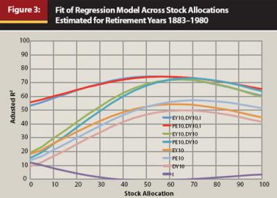
Figure 4 shows the model fit and predictions for the 30-year MWRs with a 60/40 asset allocation using EY10, DY10, and I as explanatory variables. The figure also includes confidence intervals calibrated to cover 96 percent of the historical MWRs between 1883 and 1980. Regarding the actual historical MWRs, the SAFEMAX is 3.53 percent in 1966 with this data set. MWRs ranged from a high of more than 10 percent in 1921 and 1922, to a low of less than 4 percent between 1964 and 1969. The figure illustrates as well the closeness of fit for the model predictions and the historical data. Especially since the early 1960s, the fitted values of the regression are close to the actual MWRs. Earlier, though, the fit is not always so precise. The biggest misstep occurs between 1909 and 1920, when the model predicts higher MWRs than actually observed. In four of those years, the difference was more than one percentage point. The worst prediction across the historical period occurred in 1918, when the predicted MWR was 8.14 percent and the actual MWR was 6.11 percent. This happened because EY10 was high (PE10 was low, as can be seen in Figure 2), and the MWR did not rise to the same degree as EY10. Since 1920, the difference between actual and predicted MWRs was over one percentage point in only six years. In the late 1950s, the model did not give sufficient warning for how quickly MWRs fell from their relative peak in 1949, and the model also overestimated MWRs by a small amount in 1929 and in the late 1930s. Also, the model failed to predict the full rise in MWRs in the late 1940s and early 1950s.
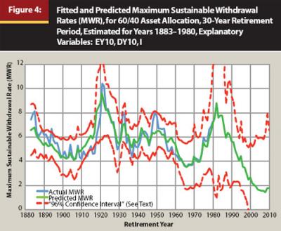
In addition to showing how the model fits the historical MWR data, the other main purpose of the figure is to provide the model predictions for MWRs in the years since 1980. The model predicts that MWRs continue rising in the early 1980s to a peak of 8.8 percent in 1982. Then they begin a long process of decline over the next 20 years. Predicted MWRs for the 60/40 asset allocation fall under 5 percent in 1992, under 4 percent in 1996, under 3 percent in 1999, and under 2 percent in 2003. EY10 experienced its lowest value in 2000, so analyses made using only that variable predict that the lowest MWR will be for the 2000 retiree. But with the income components of returns included, the worst is yet to come. The estimated MWR for the 2000 retiree is 2.7 percent, but further declines continue until 2008 when the estimated MWR reaches 1.5 percent. For 2010 retirees, it rises back only to 1.8 percent. The confidence intervals for these estimates widen dramatically in the early 1980s when bond yields rose well above previous historical experience. They narrow in the 1990s, but widen again in recent years as the values of EY10 and DY10 move out of the range of past observance. The upper limit for the confidence intervals does fluctuate around 6 percent since the 1990s, but the bottom limit is essentially at zero since 2000.
Conclusion
Given the volatility of MWRs over the years, an important question is whether retirees could have any indication of whether they were retiring at a time that would allow for a relatively high or low MWR. Market valuation and yield measures at retirement may provide a tool to help predict how much retirees can sustainably withdraw from their portfolios. The relationship between these variables and MWRs is stronger than what had first caught Campbell and Shiller’s attention regarding 10-year stock returns. The predictive power is far from perfect, and readers must ultimately judge this matter for themselves, but in my view the model fit is explained by a theoretically sound relationship likely to remain relevant in the future.
Considering that for a married couple, both age 65, there is a decent chance one spouse will live more than 30 years, and considering that administrative fees were not included in Figure 4, there is plenty to worry recent retirees. Though the 60/40 asset allocation case is the only one shown in Figure 4, the regression analysis used in this paper can provide an estimate for the maximum sustainable withdrawal rate for any combination of stocks and bonds using the values of EY10, DY10, and I at the retirement date. The reference to supplementary materials for this paper (Pfau 2011b) at the end of the article provides a URL to a basic Excel spreadsheet that allows users to input their own values for the three explanatory variables (EY10, DY10, and I) to see the predictions for MWRs across the range of stock and bond asset allocations. Recent retirees should think carefully about their rate of wealth depletion and whether their spending is on a sustainable track.
Nevertheless, it would be a great pity if recent retirees scaled down their retirement expenditures and lived a more frugal lifestyle only to find at the end that a higher withdrawal rate could have been sustainable. For this reason, these predictions must not be made lightly, and various caveats and qualifications must be taken into account. First of all, though the fitted model does closely predict actual historical outcomes, the predictions are not perfect. The adjusted R2, which indicates the preciseness of the model fit, never rises above about 75 percent. In addition, attempting to estimate the MWRs of 2000-era retirees requires less reliable, extreme out-of-sample predictions, as EY10 and DY10 were reaching all-time lows beyond anything previously experienced. If the relationships to MWRs as found in the range of previous experience do not apply when EY10, PE10, or DY10 fall outside this range, then the predicted MWRs may be overstated or understated. Changing economic circumstances may also alter the relationship between MWRs and the explanatory variables.
Furthermore, the previous worst outcomes in modern U.S. history were for retirees in the 1960s, who experienced much higher inflation than retirees in the 2000s. Inflation is specifically important for MWRs in a manner that goes beyond its impact on real asset returns, because withdrawal amounts are adjusted annually to reflect the cumulative inflation since retirement. High inflation will compound the difficulty of sustaining a real withdrawal amount. If the nominal bond yield does not provide a proper specification for inflation, then the lower inflation of today may prove material in supporting higher MWRs than the model predicts. Frankly, of course, I hope that my predictions for recent retirees turn out to be too low. But the broader point is that although the 4 percent rule could possibly work out for recent retirees, it certainly cannot be considered safe in light of the unprecedented market conditions of recent years.
Retirees must maintain flexibility, and the fixed real withdrawal strategy tested here is only a starting point to define baseline parameters about what may be sustainable. Other asset classes such as Treasury-Inflation Protected Securities (TIPS), small-capitalization stocks, international assets, real estate, commodities, annuities, and other alternative investments could all provide a way to diversify away from the risks of overvalued assets. If risky assets imply a lower withdrawal rate than can be obtained by constructing a TIPS ladder, then including TIPS in one’s retirement portfolio could help create a floor the MWR cannot fall below. Spending flexibility and reduced spending needs later in retirement could also help provide a cushion for a bad sequence of asset returns.
References
Arends, Brett. 2010. “Warning: Retirement Disaster Ahead.” Wall Street Journal (October 27).
Bengen, William P. 1994. “Determining Withdrawal Rates Using Historical Data.” Journal of Financial Planning 7, 4 (October): 171–180.
Bengen, William P. 2006. Conserving Client Portfolios During Retirement. Denver: FPA Press.
Bernard, Tara S. 2011. “With Retirement Savings, It’s a Sprint to the Finish.” New York Times (January).
Bogle, John C. 2009. Enough: True Measures of Money, Business, and Life. Hoboken, NJ: John Wiley and Sons.
Campbell, John Y., and Robert J. Shiller. 1998. “Valuation Ratios and the Long-Run Stock Market Outlook.” Journal of Portfolio Management 24, 2 (Winter): 11–26.
Cooley, Philip L., Carl M. Hubbard, and Daniel T. Walz. 2003. “A Comparative Analysis of Retirement Portfolio Success Rates: Simulations Versus Overlapping Periods.” Financial Services Review 12, 2 (Summer): 115–128.
Cooley, Philip L., Carl M. Hubbard, and Daniel T. Walz. 2011. “Portfolio Success Rates: Where to Draw the Line.” Journal of Financial Planning 24, 4 (April): 48–60.
Kitces, Michael E. 2008a. “Resolving the Paradox—Is the Safe Withdrawal Rate Sometimes Too Safe?” The Kitces Report (May).
Kitces, Michael E. 2008b. “Is the Safe Withdrawal Rate Too Safe? Or Too Aggressive!” Nerd’s Eye View blog (September 22). www.kitces.com/blog/index.php?/archives/29-is-the-safe-withdrawal-rate-too-safe-or-too-aggressive!.html.
Pfau, Wade D. 2010. “Will 2000-Era Retirees Experience the Worst Retirement Outcomes in U.S. History? A Progress Report After 10 Years.” Munich Personal RePEc Archive Paper #27107 (November).
Pfau, Wade D. 2011a. “Safe Savings Rates: A New Approach to Retirement Planning over the Life Cycle.” Journal of Financial Planning 24, 5 (May): 42–50.
Pfau, Wade D. 2011b. “Can We Predict the Sustainable Withdrawal Rate for New Retirees? Supplemental Materials” (May). http://wpfau.blogspot.com/2011/05/predict.html.
Shiller, Robert J. 2006. “Irrational Exuberance Revisited.” CFA Institute Conference Proceedings Quarterly 23, 3 (September): 16–25.