Journal of Financial Planning: April 2017
David M. Blanchett, Ph.D., CFA, CFP®, is head of retirement research at Morningstar Investment Management. He is a two-time recipient of the Journal’s Montgomery-Warschauer Award, as well as a winner of the Journal’s Financial Frontiers Award in 2007.
Executive Summary
- Optimal safe initial withdrawal rates can differ significantly across relatively similar retiree household scenarios and to a much larger extent than has been commonly noted in retirement income research. Important variables to consider are the amount of guaranteed income, the extent to which the household can adjust consumption, the risk of the investment portfolio, the return assumptions used for projections, and the degree of income stability desired by the retiree.
- Guaranteed income had the largest impact on the estimated safe initial withdrawal rates among the variables considered. Those withdrawal rates varied by more than 4 percentage points for different levels of guaranteed income.
- Although recent research using forward-looking returns suggested that 3 percent is a more appropriate safe initial withdrawal rate for retirees today, this analysis suggested that 4 percent is likely still a much better starting place for many retirees, although the optimal target varies considerably.
- For financial planners using probability of success-based metrics, targeting a lower success level (e.g., a 75 percent success rate versus a 95 percent success rate) is likely more appropriate, although the optimal target is highly dependent on retiree characteristics.
Early retirement income research focused primarily on determining the optimal safe initial withdrawal rate using a probability of success analysis where portfolio withdrawals were constant in real terms (they rose with inflation), retirement lasted for a fixed period (usually 30 years), and investment returns were based on long-term historical U.S. averages. Over time, other models were introduced to estimate the optimal initial withdrawal rate using adjusted assumptions designed to better consider the unique aspects, preferences, and behaviors of retiree households.
Despite these advances, the probability of success remains the most common approach used to determine the efficacy of a withdrawal rate strategy among financial planners today. This relatively straightforward metric (or its inverse, the probability of ruin) is calculated by dividing the number of Monte Carlo simulation runs (or scenarios) where the retirement income goal is achieved by the total number of runs considered.
A commonly noted problem with the probability of success metric is that it ignores the magnitude of failure, which can greatly affect the retiree’s consumption. It also doesn’t easily allow for the incorporation of dynamic withdrawal strategies where the portfolio withdrawal amount is adjusted throughout retirement.
The potential impact of guaranteed income on safe withdrawal rates is important given its potential impact on consumption when the portfolio fails. For example, the safe initial withdrawal rate (or amount) for a household with $100,000 in annual guaranteed income and a $1 million portfolio should not be the same as a household with $10,000 in annual guaranteed income and a $1 million portfolio, because the impact of portfolio failure on consumption is significantly different for the two households; however, this fact is typically ignored when determining safe initial withdrawal rates based on the probability of success.
This paper explored the impact of a variety of assumptions on required retirement savings levels, with an emphasis on guaranteed income and dynamic withdrawal strategies. Among the variables considered, the amount of existing guaranteed income had the largest impact on estimated safe initial withdrawal rates. This finding is especially important because the vast majority of retirement research treats the portfolio in isolation when solving for the safe initial withdrawal rate.
Safe initial withdrawal rates varied by more than 4 percentage points for varying levels of guaranteed income, from approximately 6 percent when 95 percent of wealth was in guaranteed income, versus approximately 2 percent when only 5 percent of wealth was guaranteed income. Modeling dynamic withdrawals also affected safe initial withdrawal rates, although its impact was significantly less than that of guaranteed income, slightly less than return assumptions, but greater than the assumed portfolio asset allocation.
Given the prevalence of probability of success metrics in financial planning tools, this research has important implications for retirement savers and financial planners, because a probability of success approach cannot explicitly incorporate the impact of guaranteed income or dynamic withdrawals on required retirement savings levels. Some guidance on how to incorporate this analysis into a probability of success model is provided here, and the findings suggest that when using a probability of success approach, targeting a lower success rate than those commonly used (e.g., targeting a 75 percent success rate versus a 95 percent success rate) is likely a better approach for planners today, although the true optimal success rate varied materially by the scenario analyzed.
Literature Review
Retirement research has commonly assumed that an individual, or a retiree household, desires a constant level of inflation-adjusted income during retirement. Most models assume the retiree makes all spending and investment decisions only at retirement and then follows the strategy, without adjustment, until death. This type of single-decision model is often referred to as a “static” model and was the approach taken by Bengen (1994) who introduced the well-known “4 percent rule” more than two decades ago, as well as by many other researchers, including Milevsky, Ho, and Robinson (1997), Cooley, Hubbard, and Walz (1998), and Jarrett and Stringfellow (2000) who generally supported Bengen’s initial findings, although the exact recommendations varied depending on the model and key assumptions used.
Assuming a retiree follows a static withdrawal approach significantly simplifies a retirement analysis; however, it is unlikely a retiree would actually take a static path for the entire retirement period.1 A static retirement income strategy is consistent with life cycle consumption smoothing only under a very limited set of implausible preference parameters (Milevsky and Huang 2011). In reality, a retiree whose portfolio is headed toward ruin would likely reduce withdrawals in an attempt to prolong its sustainability.
Dynamic models, which allow portfolio withdrawals to change throughout retirement, are perhaps a better reflection of decisions a retiree would make with respect to withdrawals—and the advice a client would likely receive from a financial planner throughout retirement—for at least part of retirement. The potential impact of the variety of already introduced dynamic approaches on portfolio sustainability is significant for some models. The vast majority of dynamic withdrawal strategies treat the portfolio in isolation (i.e., ignore the impact of the portfolio on consumption). This is suboptimal, because the decrease of flexibility with respect to the withdrawal is a function of the household’s other assets, such as guaranteed income.
A key assumption with a dynamic withdrawal strategy is that a retiree has the ability and the willingness to change consumption over time—that some portion of consumption is discretionary. Most retirees will likely have a retirement income goal that is a combination of discretionary and nondiscretionary needs. In other words, retirees are generally able to adjust some aspects of consumption, but not necessarily all aspects (at least without a significant degree of pain). For example, some expenses may be relatively fixed in nature, such as housing and health care, while others can more easily be adjusted, such as entertainment and transportation, and still others may be a combination of the two, like food.
Guaranteed income sources, such as public or private pension benefits and annuities, are also an important consideration given their significant role in funding retirement. For example, the U.S. first-pillar public pensions (i.e., Social Security retirement benefits) are generally the largest single income source for retirees, representing between 40 percent and 51 percent of a retiree’s aggregate income (Butrica, Iams, and Smith 2004; and Rhee 2011, respectively).
Although second-pillar employer-sponsored defined-benefit plans have been on the decline in the U.S., they still represent a significant portion of retirement assets.2 For example, of the $24.5 trillion in retirement assets at the end of Q2 2016, $8.0 trillion were in defined-benefit plans ($5.2 trillion government and $2.8 trillion private sector) and $2.0 trillion were in annuity reserves.3
This paper followed research by Finke, Pfau, and Williams (2012), who determined safe initial withdrawal rates using a utility model that incorporated survival probabilities (versus a fixed retirement period) and considered varying levels of guaranteed income for different risk aversion levels. This paper parted ways with Finke, Pfau, and Williams, though, primarily in how it assumed the investor’s risk aversion with respect to the portfolio allocation was independent of the risk associated with consumption (i.e., income stability). This paper also differs from Finke, Pfau, and Williams on how it incorporated future return projections (Finke, Pfau, and Williams used bootstrapped returns, with replacement, based on historical U.S. Ibbotson Associates series); the use of a dynamic withdrawal strategy; and by considering a more continuous potential spectrum of household states to provide more general guidance to financial planners.
Analysis
An analysis was performed to determine how varying return assumptions, levels of guaranteed income, and dynamic withdrawal strategies affect safe initial withdrawal rates. The base case scenario for the analysis was a couple, male and female, both age 65. While there were obviously considerable differences in the composition and ages of actual retiree households, a single household was considered to ease the comparison when adjusting different model parameters.
Mortality rates were based on the Society of Actuaries 2012 Immediate Annuity Mortality Table.4 This mortality table was used, rather than a more general table, such as the Social Security Administration’s 2013 Period Life Table5, to reflect the fact that individuals who receive financial planning services are much wealthier than average (Martin and Finke 2014). This is important because individuals and households with higher incomes tend to have higher life expectancies. For example, Chetty et al. (2016) noted the life expectancy of a 65-year-old in the top household income quintile was approximately three years longer than the median life expectancy. This was the same approximate increase in life expectancies when comparing the Society of Actuaries 2012 Immediate Annuity Mortality Table to the Social Security Administration’s 2013 Period Life Table for a 65-year-old.
Instead of modeling a single fixed retirement period (e.g., 30 years), the retirement model weighted the probability of the retiree household surviving to each age. As noted by Blanchett and Blanchett (2008), among others, true success is a portfolio providing income for the life (or lives) of the retiree household, not over some arbitrary fixed period. Using a fixed period does not actually model this, because it is possible for a retiree to pass away early in retirement. (The approach is discussed in additional detail in the utility model section.) To provide some perspective as to how long the retirement period would be expected to last for the base household scenario, though, there is a 43 percent chance that at least one member of the couple (or both) will survive 30 years in retirement, a 16 percent probability of surviving 35 years, and a 3 percent probability of surviving 40 years.
The guaranteed income benefit for the analysis was assumed to increase annually with inflation for the entire period of the projection. This is slightly different than how actual Social Security retirement benefits work, where the surviving spouse receives the larger of the two benefits upon the death of the first spouse (not both benefits). The approach used for this model would be most consistent with an annuity that includes a cost-of-living adjustment tied to inflation that includes a 100 percent survivor continuation benefit upon the death of the first spouse.
A portfolio fee of 50 basis points was included to reflect the expenses required to invest. The assumed fee is higher than the costs associated with investing in low-cost index mutual funds (which can be as low as about 5 basis points today), however, it is lower than the fees associated with actively managed mutual funds (which can exceed 100 basis points).
Each scenario test was based on a 1,000-run Monte Carlo projection where each run was assumed to last 50 years (i.e., to age 115 for the base case scenario). For each projection, initial withdrawal rates from 1.0 percent to 10.0 percent were considered in 0.1 percent increments (giving 91 test withdrawal rates). Taxes and required minimum distributions (RMDs) were ignored for simplicity purposes. The following subsections detail additional key assumptions for the model.
Utility model. Most retirement income research has viewed retirement consumption from a life cycle perspective, where the implied goal of a retiree (or couple) is to smooth consumption over his, her, or their retirement. This was determined primarily through an approach that either incorporates risk aversion (i.e., utility) or the likelihood of achieving some goal (i.e., the probability of success/failure). Risk aversion is a concept developed by Arrow (1965, 1971) and Pratt (1964), where the goal is to determine some level of constant consumption a person would accept in exchange for a higher average level of consumption with greater variability.
Although several utility functions are used to estimate risk aversion, the most common is a Constant Relative Risk Aversion (CRRA) utility function, shown in Equation 1, where the amount of utility (U) received varies depending on level of consumption (c) and level of investor risk aversion (y).
[1]
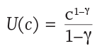
Implied within the CRRA utility function is the law of diminishing marginal utility, whereby losses (especially extreme losses) are weighted more heavily than gains. This function lends itself to retirement income modeling, because it heavily penalizes scenarios where the retiree is left destitute.6 A utility model is especially useful for retirement income modeling because it can incorporate a variety of preferences, such as a retiree’s desire to have consistent lifetime income (i.e., a preference for income stability).
The utility model used for this analysis was based on the model introduced by Blanchett and Kaplan (2013) where the risk tolerance parameter and the elasticity of intertemporal substitution (EOIS) parameter were treated as separate. This is a recursive utility approach similar to the model introduced by Epstein and Zin (1989).
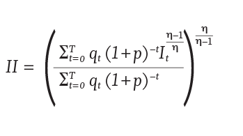
For each simulated income path, the utility-equivalent constant income level was calculated using Equation 2 where: It is the total income in year t; qt is the probability of surviving to at least year t, based on data from the Society of Actuaries 2012 Immediate Annuity Period Mortality Table; T is the length of the simulation, which is equal to 50 when t = 1 (i.e., the simulation lasts to age 115 based on the initial ages of 65); ρ is the investor’s subjective real discount rate, which is assumed to be 2 percent; and h is the elasticity of intertemporal substitution parameter.
The intertemporal substitution parameter deals the desired level of income stability during retirement. The lower the value, the more the retiree is assumed to value stable income, therefore values of 0.5, 0.25, or 0.125 were used to reflect investors with low, moderate, or high levels of income stability preference, respectively.
[2]
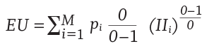
The expected utility was measured by Equation 3, where M is the number of paths; the subscript i denotes which of M paths is being referred to; pi is the probability of path i occurring, which is set to 1/M; and 0 is the risk tolerance parameter assumed to be 0.333.
[3]
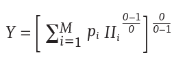
The optimal strategy, or optimal initial withdrawal rate, would be the one that maximizes the certainty-equivalent of the stochastic utility-adjusted income (i.e., maximizes Y) as noted in Equation 4.
[4]
Residual assets (i.e., bequests) were ignored in this model (i.e., the retiree household was assumed to care about maximizing retirement income).
Dynamic withdrawal model. The retirement income goal was assumed to be a combination of nondiscretionary and discretionary income goals. For the nondiscretionary portion of the income goal, the annual income need was assumed to increase annually based on inflation. This withdrawal amount was fixed regardless of the ongoing sustainability of the withdrawal amount (i.e., even if the portfolio was headed for certain ruin, that amount would still be withdrawn). The nondiscretionary income portion was the same as the static approach common in past retirement research.
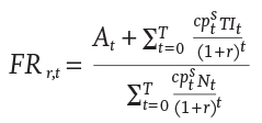
For the discretionary portion of the income goal, the annual withdrawal was determined so that the funded ratio for the retiree was constant throughout retirement for that run. The funded ratio (FR) was calculated using Equation 5, where T is the total number of simulation years, which is equal to 50 when t = 1; At is total assets (portfolio value) at year t; cpts is the cumulative probability of surviving to year t (and is based on the retiree household composition); TIt is total annual income from all sources (i.e., total guaranteed income and portfolio income) at year t; Nt is the annual income goal (need) at year t, which is the total income spent in the respective year; and r is the discount rate, which is the real return on bonds for the first 20 years of the projection (all calculations in the analysis are in real terms).
[5]
The withdrawal amount was determined for each year of a given run so that the funded ratio was constant throughout the run. Using this approach, if the portfolio experienced a negative (or poor) return, the funded ratio decreased. To get the funded ratio back to its target, the portfolio withdrawal amount would need to decrease, in real terms. The maximum annual change in the withdrawal amount was assumed to be 5 percent (positive or negative, in real terms).
The withdrawal was assumed to never increase beyond the initial withdrawal amount (increased by cumulative inflation). While other dynamic withdrawal strategies do allow for withdrawals to potentially increase if the portfolio outperforms, this analysis assumed that even for the dynamic portion of the goal the income would not exceed the original target increased by inflation. This approach therefore, was focused primarily on maximizing the initial withdrawal rate with less of an emphasis on increasing withdrawals during retirement. Given the constraints in the approach (i.e., the maximum annual change in the withdrawal amount was 5 percent) it was technically possible for the portfolio to run out of money, which isn’t always a possibility in dynamic models.
Figure 1 provides insight into how the annual withdrawals would differ from a portfolio with a 40 percent equity allocation, assuming a 4 percent initial withdrawal rate using a static withdrawal model (Panel A), versus a dynamic withdrawal model (Panel B).
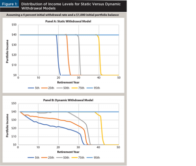
Panel A of Figure 1 demonstrates how static models result in early and abrupt failure for retirees. For the worst 1 in 20 runs (i.e., the 5th percentile), the portfolio value went to $0 by the 21st year of retirement. For more than half of the runs in Panel A, the portfolio reached $0 by the 31st year of the projection (this would suggest the probability of funding retirement income was approximately 50 percent). In contrast, using the dynamic model (Panel B), the portfolios tended to last much longer, but the income level may be reduced based on portfolio returns. For example, at the 5th percentile outcome (worst 1 in 20), the income lasted until year 33 in the dynamic model (Panel B), but the withdrawal amount had been cut in half by year 23.
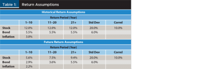
Return assumptions. The analysis used two sets of returns, historical and forecasted. Historical returns were based on the approximate long-term average returns of U.S. stocks and bonds using the Ibbotson® SBBI® time series data since 1926. The forecasted returns were based on Morningstar Investment Management LLC’s 2016 capital market assumptions. These forecasted returns were time-varying, where returns in the near-term, in early retirement, were assumed to be relatively low to reflect current market conditions, although they were assumed to increase throughout time (i.e., drift back toward the long-term average). The historical returns were not assumed to be time-varying; they were constant over the entire projection. For simplicity purposes, the standard deviations and correlation values were the same for both sets of assumptions. There was no assumed serial correlation for the returns. The assumptions for the respective series are included in Table 1.
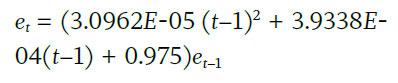
Equity allocation glide path. The equity allocation (e) for the first year of retirement (t) was specified at either 10 percent, 40 percent, or 70 percent. The equity allocation was assumed to decline each year during retirement consistent with the rate of change in the equity allocations for the Morningstar Lifetime Indexes.7 Despite debate regarding the efficacy of declining glide paths during retirement, this remains the most common shape among retirement income products today. Equation 6 was used to determine the equity allocation, with annual rebalancing back to the target allocation.
[6]
This approach treated the risk aversion associated with the portfolio as separate from the risk aversion associated with income. Although the two may likely be related for some investors, other retirees will be willing to take substantial risk in their portfolio but may be far more risk averse with respect to funding retirement. This model allowed for these varying preferences.
Results
A common metric for determining safe initial withdrawal rates, especially among financial planners, is the probability of success. Table 2 compares the results of the utility model to the results of a more traditional probability of success model. Table 2 includes the probability of success for various initial withdrawals (3 percent to 6 percent in 0.5 percent increments) for varying retirement periods (20 to 40 years in five-year increments), for various initial equity allocations (10 percent, 40 percent, and 70 percent), based on either the historical or forecasted return models. The withdrawals were assumed to be constant in real terms over the period (i.e., based on a static withdrawal method).
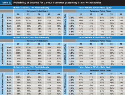
Table 2 has several important takeaways. First, the safe initial withdrawal rate varied significantly by scenario assumptions. For example, although 4 percent has been commonly cited as a safe initial withdrawal over 30 years using historical returns, a 5.5 percent initial withdrawal rate has been relatively safe for a 20-year retirement period, and a 3.0 percent initial withdrawal rate appeared to have been more reasonable over a 40-year retirement period. Also, changing the returns projection method from historical to projected (i.e., using lower returns) had a significant, negative impact on the safe initial withdrawal rate. For example, based on the 40 percent initial equity allocation, the probability of success of a 4 percent initial withdrawal rate over a 30-year retirement period was 92 percent using the historical returns model, but fell to 53 percent using the forecasted model. This reduction in the probability of success was similar to the findings by Blanchett, Finke, and Pfau (2013), among others.
Using more realistic return estimations significantly affected required savings rates. Moving to a forward-looking model while keeping the probability of success approximately equal over a 30-year retirement period required the initial safe withdrawal rate to drop to 3 percent from 4 percent. This 1 percentage point drop in the safe withdrawal rate resulted in a required savings multiplier of 33.33 (1/3 percent = 33.33) times the required income goal.
Table 3 includes the safe initial withdrawal rates estimated using the utility model introduced in the analysis section, based on various income stability preferences (low, moderate, and high), levels of guaranteed income as a percentage of total wealth (5 percent, 25 percent, 50 percent, 75 percent, and 95 percent), percentage of the income that was assumed to be nondiscretionary (from 0 percent to 100 percent in 25 percent increments), and returns (either historical or forecasted).
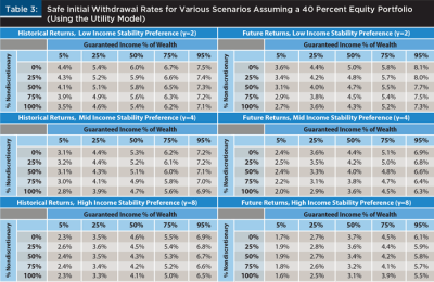
To provide some context to understand the “guaranteed income as a percent of wealth” variable in Table 3, retirement wealth was assumed to consist of two assets: guaranteed income and the portfolio. Each dollar of guaranteed income had a mortality-weighted net present multiple of 24.23, which is the present value of $1 of inflation-adjusted income for life, weighted by mortality. For example, if a retiree household expected $50,000 in annual inflation-adjusted guaranteed income, the value of the benefits would be $1,211,444 ($50,000 x 24.23 = $1,211,444). If that household had retirement savings of $500,000, then the total value of the guaranteed income would be 70.78 percent of the total wealth for that household ($1,211,444/$1,711,444 = 70.78 percent). Other assets that could potentially be used to fund retirement, most notably home equity, are ignored in this analysis.
Using a traditional probability of failure analysis with a static withdrawal approach (the approach used to estimate the values in Table 2), the safe initial withdrawal rates in each of the six grids in Table 3 would be identical. However, introducing nondiscretionary spending, and especially the existing level of guaranteed income, significantly impacted the safe initial withdrawal rate.
Varying levels of guaranteed income shifted the safe initial withdrawal rate approximately 4 percentage points on average (from approximately 6 percent when 95 percent of wealth was in guaranteed income, versus approximately 2 percent when only 5 percent of wealth was in guaranteed income). In contrast, varying levels of nondiscretionary spending tended to shift withdrawal rates by approximately 50 basis points (holding the level of guaranteed income constant). Moving to a forecasted returns model lowered the safe withdrawal rates by approximately 1 percent, on average.
The results in Table 3 also provide guidance on how the potential value of an annuity could differ for households with different levels of existing guaranteed income. A household with relatively little guaranteed income could potentially benefit far more from an annuity than a household with a high level of guaranteed income, given the significantly lower initial safe withdrawal rates (e.g., about 3 percent). This is especially true for retirees with higher income stability preferences and more conservative portfolios.
Table 4 shows how safe initial withdrawal rates vary based on different initial portfolio allocations assuming a moderate income stability preference.
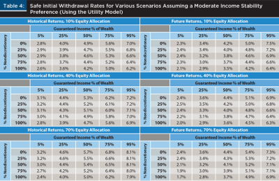
Similar to the probability of success analysis results in Table 2, safe initial withdrawals tended to increase for more aggressive portfolios, although the changes across portfolio levels weren’t nearly as great as changes in the level of existing guaranteed income for the retiree household. This suggests that, while the portfolio allocation was important when determining the safe initial withdrawal rate, other assumptions are likely to impact the results significantly more.
Equivalent Probability of Success Target
The previous analysis demonstrated that safe withdrawal rates differed significantly based on key assumptions. Some assumptions, such as the retiree’s desire to have more or less safety with respect to the retirement income goal, can already be incorporated in a financial planner’s recommendations relatively easily today. Other assumptions, though, such as the level of guaranteed income, may not affect the required savings (i.e., safe withdrawal rate) recommendation, especially if the outcomes metric used by the financial planner’s modeling software is the probability of success.
Although the utility framework may result in better estimates of minimum safe withdrawal rates, the vast majority of financial planners are unlikely to be able to implement the framework with clients. Therefore, it is worth providing guidance on how to adapt the previous findings into outcomes metrics commonly used by financial planners today, such as the likelihood of accomplishing a goal (i.e., the probability of success).
One approach to convert the previous findings into results that can be estimated using more common models is to determine the probability of success that would yield the same result for a respective
scenario. For example, according to Table 3, a retiree with moderate income stability preference invested in a 40 percent initial equity allocation with 50 percent of the retirement income need being nondiscretionary and 50 percent of wealth in guaranteed income, would have a 4.0 percent initial safe withdrawal rate estimated using forecasted returns (it would be 5.1 percent using historical returns). To achieve the same initial safe withdrawal rate (4.0 percent) based on a probability of success analysis using similar assumptions (portfolio allocation, future returns, a 30-year retirement period, etc.), the target probability of success would need to be 36 percent. In other words, targeting a probability of success of 36 percent would result in the same initial safe withdrawal rate (4.0 percent) based on that set of assumptions.
Table 5 provides some additional perspective on how target success rates varied across scenarios in order to achieve the same initial withdrawal rates noted in Table 3 (which were estimated using the previously introduced utility model), assuming a 30-year retirement period.
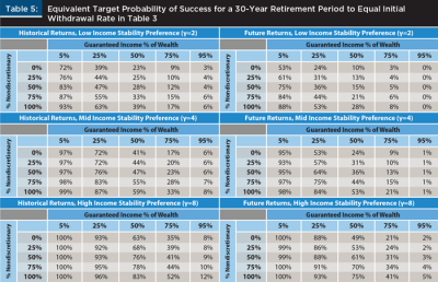
The target probabilities of success were much higher for those scenarios where guaranteed income was a smaller percentage of the retiree’s total wealth. This should not be surprising given the previously estimated safe initial withdrawal rates were much lower for lower levels of guaranteed income. One implementation issue associated with the results in Table 5 was the dispersion of potential target success rates, which ranged from 0 percent to 100 percent, depending on the scenario.
An important takeaway from Table 5 is that targeting a very high probability of success (e.g., 95 percent) will not likely be optimal for most households. Although targeting a high probability of success creates a perception of safety, it appears that for most retirees it may lead to initial safe withdrawal rates that are too safe, especially for those households with high levels of existing guaranteed income. Therefore, although it may be difficult to explain why targeting 75 percent (or even 50 percent) is actually quite safe (versus 95 percent), not doing so will likely result in below-optimal consumption during retirement.
Relative Impact Analysis
The results of the analysis demonstrated that safe initial withdrawal rates can vary considerably by household scenario. To provide some insight into the relative impact of different assumptions, an ordinary least squares (OLS) regressions was performed where the dependent variable was either target probability of success for an assumed 30-year retirement period that would result in the same safe initial withdrawal rate using the utility model as a probability success analysis (Panel A of Table 6, the same approach used to estimate the values in Table 5), or the actual initial safe withdrawal rate (Panel B of Table 6), where the independent variables were guaranteed income as a percentage of total wealth, the percentage of the total retirement need that was nondiscretionary, income stability preference (–1 if low, 0 if moderate, 1 if high), portfolio equity allocation, and return assumptions (dummy variable, which equals 0 if historical returns and 1 if forecasted returns). The results are included in Table 6.
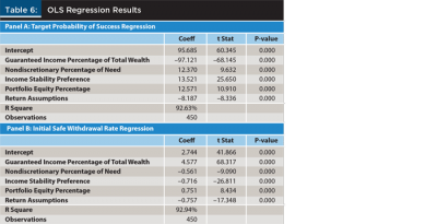
The R-squared measures of both OLS regressions were relatively high (about 92 percent), which suggests both regressions explained a significant portion of the variance of the respective dependent variables. A simulation based on the unique client data would be a more robust way to estimate safe withdrawal rates, for example, however, it appears possible to approximate the respective values with a reasonable degree of accuracy. Blanchett (2013) took this approach.
Here is an example to illustrate how to read Table 6: assuming a retiree household (male/female, both age 65, which is the base scenario for this analysis) with 50 percent of the retirement need covered from guaranteed income, where 80 percent of the income need is nondiscretionary, with a moderate income stability preference, a 40 percent initial equity allocation, and using forward-looking returns, the initial safe withdrawal rate would be 4.2 percent (using coefficients in Panel B, the actual value from Table 3 for this scenario is 4.0 percent). This 4.2 percent initial safe withdrawal rate was estimated using the utility model introduced earlier, but it could also be estimated using a traditional probability of success analysis, targeting a 30-year retirement period using future returns with a 54 percent target probability of success.
A 54 percent target probability of success is significantly lower than success levels typically targeted by financial planners (at least based on the author’s experience), and the resulting 4.2 percent initial safe withdrawal rate is significantly higher than recent research incorporating forecasted returns would suggest. However, the fact that the household has a relatively large amount of guaranteed income provides an important buffer should the portfolio actually fail. Because retirement income modeling is focused on consumption, incorporating guaranteed income is a critical component.
Conclusions
To better serve retirees and those saving for retirement, financial planners need to move beyond heuristic-based initial safe withdrawal rates. Results from this analysis suggest that optimal initial safe withdrawal rates varied significantly when guaranteed income was considered, from approximately 6 percent when 95 percent of wealth was in guaranteed income, versus approximately 2 percent when only 5 percent of wealth was in guaranteed income.
Safe initial withdrawal rates also varied when using dynamic withdrawal strategies and forward-looking investment return projections, but the impact was more muted (less than 1 percentage point).
This analysis also suggests that metrics such as the probability of success will likely paint an incomplete picture with respect to optimal levels of retirement savings, since probability of success measures generally ignore the magnitude of failure and cannot incorporate withdrawal adjustments over time. Although adopting a utility model might not be practical for all financial planners, this paper introduced a way to adapt a probability of success approach to approximate the results of the utility model.
Overall, the analysis here suggests that targeting a lower success level (e.g., a 75 percent success rate versus a 95 percent success rate) is likely more appropriate, although the optimal target is highly dependent on the retiree scenario.
Endnotes
- This also ignores the possibility of some type of future shock to the household, which is likely to happen but difficult to model.
- See the Employee Benefit Research Institute’s “FAQs about Benefits—Retirement Issues,” at ebri.org/publications/benfaq/index.cfm?fa=retfaq14.
- The remaining $14.5 trillion were in either IRAs or defined contribution plans. See data from the Investment Company Institute at www.ici.org/research/stats/retirement/ret_16_q2.
- See naic.org/store/free/MDL-821.pdf.
- See ssa.gov/oact/STATS/table4c6.html.
- A minimum level of guaranteed income is always included to eliminate the possibility of an infinite marginal utility at zero income.
- See corporate.morningstar.com/us/documents/Indexes/AssetAllocationsSummary.pdf.
References
Arrow, Kenneth J. 1965. “Aspects of the Theory of Risk Bearing.” Yrjö Jahnsson Lectures. Yrjö Jahnsson Foundation, Helsinki.
Arrow, Kenneth J. 1971. Essays in the Theory of Risk Bearing, Vol. 1, Chicago: Markham Publishing Company.
Bengen, William P. 1994. “Determining Withdrawal Rates Using Historical Data.” Journal of Financial Planning 7 (4): 171–180.
Blanchett, David M. 2013. “Simple Formulas to Implement Complex Withdrawal Strategies.” Journal of Financial Planning 26 (9): 40–48.
Blanchett, David M. and Brian C. Blanchett. 2008. “Data Dependence and Sustainable Real Withdrawal Rates.” Journal of Financial Planning 21 (9): 70–85.
Blanchett, David M., Michael Finke, and Wade D. Pfau. 2013. “Low Bond Yields and Safe Portfolio Withdrawal Rates.” The Journal of Wealth Management 16 (2): 55–62.
Blanchett, David, and Paul Kaplan. 2013. “Alpha, Beta, and Now…Gamma.” The Journal of Retirement 1 (2): 29–45.
Butrica, Barbara, Howard Iams, and Karen Smith. 2004. “The Changing Impact of Social Security on Retirement Income in the United States.” Social Security Bulletin 65 (3).
Chetty, Raj, Michael Stepner, Sarah Abraham, Shelby Lin, Benjamin Scuderi, Nicholas Turner, Augustin Bergeron, and David Cutler. 2016. “The Association between Income and Life Expectancy in the United States, 2001– 2014.” JAMA 315 (16): 1,750–1,766.
Cooley, Philip L., Hubbard, Carl L. and Daniel T. Walz. 1998. “Retirement Savings: Choosing a Withdrawal Rate that Is Sustainable.” Journal of the American Association of Individual Investors 20 (2): 16–21.
Epstein, Larry G. and Stanley E. Zin. 1989. “Substitution Risk Aversion and the Temporal Behavior of Consumption and Asset Returns: A Theoretical Framework.” Econometrica 57 (4): 937–969.
Finke, Michael, Wade Pfau, and Duncan Williams. 2012. “Spending Flexibility and Safe Withdrawal Rates.” Journal of Financial Planning 25 (3): 44–51.
Jarrett, Jaye C. and Tom Stringfellow. 2000. “Optimum Withdrawals from an Asset Pool.” Journal of Financial Planning 13 (1): 80–93.
Martin, Terrance, and Michael Finke. 2014. “A Comparison of Retirement Strategies and Financial Planner Value.” Journal of Financial Planning 27 (11): 46–53.
Milevsky, Moshe A. and Huaxiong Huang. 2011. “Spending Retirement on Planet Vulcan: The Impact of Longevity Risk Aversion on Optimal Withdrawal Rates.” Financial Analysts Journal 67 (2): 45–58.
Milevsky, Moshe Arye, Kwok Ho, and Chris Robinson. 1997. “Asset Allocation via the Conditional First Exit Time or How to Avoid Outliving Your Money.” Review of Quantitative Finance and Accounting 9 (1): 53–70.
Pratt, John W. 1964. “Risk Aversion in the Small and in the Large.” Econometrica 32: 122–136.
Rhee, Nari. 2011. “Meeting California’s Retirement Security Challenge.” U.C. Berkeley Labor Center, available at laborcenter.berkeley.edu/meeting-californias-retirement-security-challenge.
Citation
Blanchett, David M. 2017. “The Impact of Guaranteed Income and Dynamic Withdrawals on Safe Initial Withdrawal Rates.” Journal of Financial Planning 30 (4): 42–52.