Journal of Financial Planning: April 2012
Wade D. Pfau, Ph.D., CFA, an associate professor at the National Graduate Institute for Policy Studies in Tokyo, Japan, holds a doctorate in economics from Princeton University. His hometown is Des Moines, Iowa. (wpfau@grips.ac.jp)
Acknowledgments: I am grateful for financial support from the Japan Society for the Promotion of Science Grants-in-Aid for Young Scientists (B) #23730272.
Executive Summary
- Although most everyone would agree that stock valuations matter, the question remains whether clients with a long-term outlook (such as those planning for retirement) can hope to act successfully on information about valuations.
- This article provides favorable evidence based on the historical record for long-term investors to obtain improved retirement planning outcomes (lower savings rates, higher withdrawal rates) using valuation-based asset allocation strategies.
- A specific example compares a 50/50 fixed allocation strategy with a Benjamin Graham and David Dodd-inspired valuation-based strategy with a stock allocation of 25 percent, 50 percent, or 75 percent, determined by the value of the cyclically adjusted price-earnings ratio with respect to its median value up to that point in history.
- Important caveats are discussed. But even if clients or advisers decide against adopting valuation-based asset allocation, advisers may at least be able to use the research findings to help persuade clients to stay the course and not give in to the temptation to change their asset allocation in the “wrong direction,” such as increasing stock holdings after valuations rise or panicking and selling stocks after a plummet in valuations.
In an interview for the December 2011 Journal of Financial Planning, Lance Ritchlin asked William Bengen, “What do you see as the next step regarding research into safe withdrawal rates?” Bengen replied, “I think that was something … where you vary, now, the investment approach based on some criteria that have yet to be defined, whether it be value or something else.… I think all the research done has pretty much assumed a portfolio with a pretty constant stock-bond ratio throughout the whole time of the client’s retirement.” I will provide an attempt to fulfill Mr. Bengen’s research suggestion. I investigate the role of a valuation-based asset allocation strategy for a client’s accumulation and retirement phases. Such an approach is not unknown to readers of the Journal—in the same December issue, Solow, Kitces, and Locatelli (2011) investigate how these sorts of strategies improve risk-adjusted returns.
Based on previous work described in Campbell and Shiller (1998) and other research papers, Shiller (2000) popularized the notion that valuation ratios, specifically a cyclically adjusted P/E ratio equal to price divided by average real earnings over the previous 120 months (PE10), can provide predictive power for long-term real stock market returns. Checking the relationship between PE10 and subsequent 10-year real stock returns with updated data reveals that PE10 explains 30.2 percent of the variation in these subsequent returns. The explanatory power increases to as much as 60 percent for 19-year average real stock returns. Because such regressions are estimated using overlapping observations, as the same year data point is used in the construction of both variables over multiple periods, scholars have subsequently debated whether the relationship is statistically significant. Shiller (2000) provides a review of this literature. More generally, economists often worry more about statistical significance than economic significance, and Shiller (2010) understands this point when he writes, “A regression would not indicate a terribly good fit, but it is a good enough fit to suggest that there is something to this model.”
In seeking to determine the economic significance of this relationship, this research explores whether otherwise passive long-term investors can exploit it to obtain improved retirement planning outcomes in comparison with a fixed asset allocation strategy with the same average allocation to stocks. Strategic asset allocation involves deciding on an allocation to properly balance risk and return objectives after considering factors such as capital market expectations, age, job stability, existing wealth, planned expenditures, risk tolerance, and other factors affecting the willingness and ability to bear risk. Although most agree that stock valuations matter, the real question is whether clients with long-term horizons can act successfully on information about valuations. Should stock market valuations, through their effect on capital market expectations, be added to the list of characteristics clients consider when determining their asset allocation?
The long-term focus is important. Market valuation levels tend to revert to their average over long periods. Though testing the statistical significance of that statement is complex, Campbell and Shiller (1998), Tomlinson (2010), and Pfau (2011a) all provide types of evidence for this. When PE10 is low, markets tend to exhibit mean reversion, and relatively higher future returns can be expected. But because the precise timing of this mean reversion is not known in advance, and is indeed random, expecting the result to happen in the short term will not be possible. This research is indeed grounded in the notion that attempting to beat the market in the short run is futile. It can take years for mean reversion to happen. But can patient clients find a strategy to take advantage of this mean reversion in market valuation levels?
As a case study, I will compare a fixed 50/50 asset allocation strategy with a strategy introduced by Graham and Dodd (1940) in which investors maintain a 50/50 asset allocation when valuations fall within a range between 2/3 and 4/3 of their historical average value; the stock allocation is 75 percent when valuations are less than 2/3 of their average and 25 percent when valuations are more than 4/3 of their average. These numerical bounds correspond to evolving PE10 values of approximately 10 and 21 over time. I will demonstrate the potential for valuation-based asset allocation strategies to increase the Bengen (1994) style worst-case scenario SAFEMAX withdrawal rate as well as maximum sustainable withdrawal rates in general, to decrease the savings rate needed to meet a wealth accumulation target at retirement, and to decrease the Pfau (2011a) style “safe” savings rate needed to meet one’s retirement spending goals without worrying about the implied wealth accumulation or withdrawal rate. I will demonstrate historical success for valuation-based strategies.
My claim for historical success will be controversial, at least as to whether I have effectively avoided look-back bias, whether taxes and transaction costs would overturn the results, and whether such success will continue in the future. Nevertheless, at least for clients inclined to adjust their allocation in response to market events, the sorts of mechanical rules outlined here would provide a better alternative than emotion-based and arbitrary market-timing decisions. Generally, investors tend to give in and increase stock allocations near a market peak and then panic and decrease allocations after a market drop. Evidence for this can be found in studies such as Barber and Odean (2000), Frazzini and Lamont (2008), and DALBAR’s annual Quantitative Analysis of Investor Behavior. It is the opposite of what should happen. Jenkins (1961) argues that formulaic rules, “most certainly help to protect the investor against the dangers of emotionalism, and offer a guide to action that can protect him from acting under the perhaps unwise impulse of the moment.” Incorporating valuation-based asset allocation into an investment policy statement could provide the psychological resolve to weather big market drops, especially as such drops tend to occur when valuations are high, and so the investor would already be at a lower stock allocation.
Literature Review
Jenkins (1961) reviews the history of stock formula investing plans, which obtained great popularity between the 1930s and 1950s. Some of these formula plans are still extremely popular today, such as dollar-cost averaging, buy and hold (which implies not rebalancing), and the constant-ratio plan, which today is better known as buy and hold with periodic rebalancing either at specific time intervals or when deviations from the targeted asset allocation become sufficiently large. Here, I refer to constant-ratio plans as “fixed allocation.”
In this research, I update into modern form a type of formula plan that Jenkins might have included in his chapter on variable-ratio plans. These plans were based on trend lines, moving averages, and intrinsic values. Their underlying theme was that stock markets tend to exhibit cyclical patterns over time. Stock allocations should increase when stock prices/values are relatively low, and allocations should decrease when prices/values are relatively high. Or, as Lucille Tomlinson (1953) describes, “A variable ratio formula provides for smaller percentages of stocks in high market areas, where the risk of owning stocks is greatest, and for larger percentages in low market areas, where the risk of loss is bound to be considerably less.” More generally, stock formula plans were meant to guide investors with mechanical rules to prevent behavioral mistakes.
Though earlier writers were investigating asset allocation strategies that real people might consider using, an unfortunate detour in much of the recent research about “market timing” has been to compare only a 100 percent stocks fixed allocation strategy against a strategy switching between 100 percent stocks and 100 percent cash as dictated by the timing rule in which changes are made even when the market is just slightly above or slightly below its “fair valuation level.” Studies considering only extreme allocation choices include Smithers and Wright (2000) and Stein and DeMuth (2003), who find supporting evidence for timing, and Fisher and Statman (2006) and Blanchett (2011), who find opposing evidence for timing.
Focusing on the negative studies, Fisher and Statman (2006) is one of the few extant studies providing counter evidence to the idea that a market-timing strategy guided by existing valuation measures with relatively few trades made over a long period can improve risk-adjusted investment returns. However, their investigation is limited by their comparison of the above-mentioned extreme strategies. One hundred percent stocks is a rather volatile benchmark for comparison that is usually not used by conservative household investors. Ex ante, it also has a much higher average stock allocation than the timing strategies. It is important too that the extreme market-timing strategies they consider fail to hedge against the possibility that valuations can deviate from their average levels for extended periods. As for Blanchett (2011), the timing decisions are made randomly, and the Monte Carlo simulation produces returns that are independent over time, leaving no role for valuation feedback. This will not be convincing to anyone who believes that valuations may be beneficial in predicting long-term returns.
Responding, in particular, to the Fisher and Statman study, Pfau (2012) finds that most every permutation of valuation-based asset allocation strategies based on PE10 demonstrates strong potential to improve risk-adjusted returns for conservative long-term investors. Such valuation-based strategies provide comparable returns as 100 percent stocks, but with substantially less risk according to a wide variety of risk measures. Meanwhile, valuation-based strategies provide comparable risks and the same average asset allocation as a 50/50 fixed allocation strategy, but with much higher returns. When comparing the absolute returns for different strategies, the 50/50 fixed allocation strategy provides a more suitable benchmark, as it allows for comparisons between strategies with similar risk and the same average stock allocation.
Having already implicitly understood the need for more suitable comparison groups and more realistic allocation choices, Solow, Kitces, and Locatelli (2011) is another study arguing that valuation-based strategies can improve risk-adjusted returns. Though they may have overstated the case for statistical significance by not considering that their data observations are overlapping rather than independent, they do provide a compelling case that capital market expectations do differ dramatically between high and low valuation environments.
The above studies describe the situation for the accumulation phase. For retirement decumulation, Kitces (2008) and Pfau (2011b) both use fixed asset allocations to explore the relationship between retirement date valuations and sustainable withdrawal rates. Kitces (2008) argues that safe withdrawal rates are higher when valuations are low. Pfau (2011b) extends this idea with a regression model also including dividend yields and bond yields to show that historically a close relationship has existed between sustainable withdrawal rates and these variables. We can obtain fairly reasonable predictions for the sustainable withdrawal rate based on market conditions at the retirement date. If valuations affect withdrawal rates when using a fixed asset allocation, the next reasonable step is to consider the impact of changing allocations in response to valuations. Kitces (2009) does investigate the impact of valuation-based strategies on sustainable withdrawal rates, arguing that incorporating valuations into asset allocation decisions can help increase the safe withdrawal rate.
Methodology and Data
I use a historical simulations approach, considering the perspective of clients retiring in each year of the historical period. An individual saves for retirement during the final 30 years of her career, and she earns a constant real income in each of these years. A fixed savings rate determines the fraction of this income she saves at the end of each of the 30 years. Retirement begins at the start of the 31st year, and the retirement period is assumed to last for 30 years. The accumulation and decumulation life cycle is 60 years. Withdrawals are made at the beginning of each year during retirement. Withdrawal amounts are defined as a replacement rate from final preretirement salary and are adjusted for inflation in subsequent years. I assume that the client wishes to replace 100 percent of her final salary with withdrawals from her accumulated wealth. Because this does not account for Social Security, other income sources, or the fact that savings reduce preretirement expenditures, this replacement rate is surely much too high for most everyone. As a result, the suggested savings rates are unrealistically high. But this is not a problem. The savings rates I find resulting from this assumption can simply be multiplied by a fraction to obtain any other replacement rates (multiply the savings rate by 0.50 for a 50 percent replacement rate, for instance).
Robert Shiller’s website (www.econ.yale.edu/~shiller/data.htm) provides the data. From his spreadsheet, investment portfolios include large-capitalization stocks (Standard and Poor’s Composite Stock Price Index) and short-term fixed-income assets (annual yield from six-month commercial paper rates). Real results are obtained by adjusting for the inflation measure in Shiller’s data set, which is the Consumer Price Index-All Urban Consumers for years since 1913.
The investment portfolio is rebalanced to the targeted asset allocation at the start of each year. With these 139 years of data, I consider 30-year careers followed by retirements beginning in the years 1901 to 2010. In addition, I consider 30-year retirements beginning between 1871 and 1980. In considering a 60-year life cycle with 30 years of work followed by 30 years of retirement, there are 80 overlapping periods with retirements beginning between 1901 and 1980.
The PE10 measure is the stock price in January divided by the average real earnings on a monthly basis over the previous 10 years. Campbell and Shiller (1998) justify this measure as a way to remove cyclical factors from earnings. The concept derives from Graham and Dodd (1940), who said, “The period for averaging earnings would ordinarily be 7 to 10 years.” PE10 has become a widely accepted valuation measure despite lacking a precise theoretical underpinning for the choice of 10 years, and so I use it to avoid look-back bias in case another definition provides even stronger results. Solow, Kitces, and Locatelli (2011) suggest instead using five years of earnings (PE5).
There are infinite ways for creating a formula plan, with various choices to be made about how to change asset allocations and which valuation indicators to use for decision rules. Look-back bias is a real problem, as it could be easy to keep searching for a formula plan that works with the historical data but would not necessarily have been chosen in advance. There are three ways to try to limit such bias: choose a formula plan created long ago, decide on the formula parameters in advance before looking at the data, and check for robustness by confirming the results for many different plan variations. Though more frequent action is possible, I only consider clients who check whether a revision for their asset allocation is required at the beginning of each year.
I will illustrate this concept with one valuation-based strategy. Having looked at many permutations, some aspects of this strategy (such as using the rolling historical median to define fair value PE10) were chosen specifically because they result in the worst wealth accumulations for the valuations strategy. The strategy I illustrate is representative of what can be expected and is not chosen because it provides a misleadingly positive portrait. Pfau (2012) shows results for many other strategies during long accumulation periods.
The strategy considered here is inspired by Graham and Dodd (1940). They suggest that a neutral 50/50 strategic allocation be maintained as long as PE10 falls within a band between 2/3 and 4/3 of its historical average. I define the historical average as the rolling median between the start date and that point in history. This is a plausible choice, and ex post, it also performs relatively poorly, providing a further check against look-back bias. More extreme allocations are used only when PE10 moves outside these bounds, with a 25 percent stock allocation when PE10 is high and a 75 percent stock allocation when PE10 is low. Asset allocation changes can be made by directing new contributions and by rebalancing.
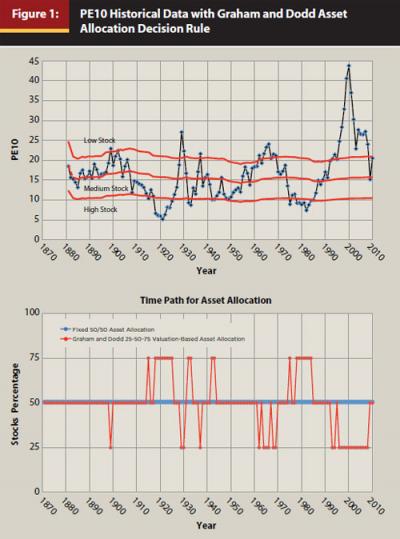
Figure 1 shows PE10 along with the bounds for the Graham and Dodd decision rules, as well as the corresponding asset allocation for each year in the historical record. Between 1871 and 1914, both strategies shared the same allocation in every year except 1899 (PE10 cannot be calculated until 1881 because 10 years of data are needed, so I assume the valuation-based strategy uses 50/50 for 1871–1880). This explains why the outcomes will be quite similar during the early part of the historical period. Between 1915 and 1944, the asset allocation does change rather frequently. For 1944 through 1961, both strategies share the same allocation. For 6 years in the 1960s, the valuation-based strategy uses a lower stock allocation, and from the mid-1970s to mid-1980s, the tendency is toward a higher stock allocation. From 1985 through 1992, the allocations were again the same, and then as the market boomed in the 1990s the valuations strategy uses a lower stock allocation for all years between 1993 and 2008, except for 1995. Over the historical period, there were 28 allocation changes, for an average of one change every five years.
Valuation-Based Asset Allocation and Maximum Sustainable Withdrawal Rates
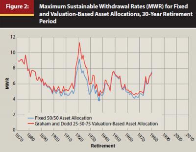
Figure 2 shows the historical maximum sustainable withdrawal rates (MWRs) for 30 years of inflation-adjusted withdrawals with a fixed 50/50 and a Graham and Dodd 25-50-75 valuation-based asset allocation strategy. MWRs vary among studies because of differences in data sets, asset allocations, fees, when during the year withdrawals are made, and other matters. In Figure 2, the SAFEMAX worst-case withdrawal rate occurred for both strategies in 1937. With a fixed 50/50 strategy, the SAFEMAX was 3.93 percent. With the valuation-based strategy, the SAFEMAX was 0.65 percentage points more at 4.58 percent. If the SAFEMAX is the criterion used to define a “safe withdrawal rate,” then the valuation-based strategy would offer conservative retirees the opportunity to raise their portfolio spending by nearly 17 percent. Another low point occurred for 1966 retirees, when the 50/50 fixed strategy supported a 4.14 percent withdrawal rate, compared with 4.6 percent for the valuation-based strategy. More generally, the valuation-based strategy supports equally high or higher withdrawal rates over 30-year retirements across the historical period, with differences of more than 2 percentage points in a few years. People retiring in 1979 and 1980 provide the only exceptions, as by then, the underperformance of the valuation-based strategy during the prolonged market boom with soaring valuations in the 1990s began to show its effect. Nevertheless, the underperformance of the valuation-based strategies in those two years is not critical—both strategies supported relatively high withdrawal rates of more than 7 percent.
Valuation-Based Asset Allocation and Savings Rates to Meet a Wealth Accumulation Target
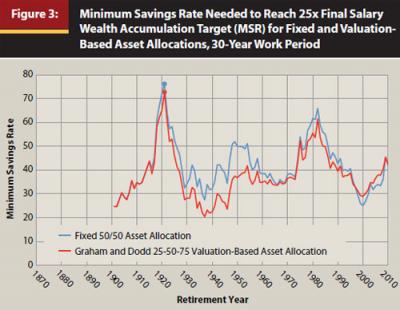
Next, consider the savings rate (MSR) needed over a 30-year career to achieve a wealth accumulation target of 25 multiples of constant real salary by retirement. This would be the amount needed for traditional retirement planning to use a “safe” 4 percent withdrawal rate if the goal is to replace 100 percent of a client’s preretirement income. Again, this replacement rate is surely too high, but planners can multiply the savings rates shown by the appropriate fraction to obtain the savings rate for any desired replacement rate. Figure 3 shows that the valuation-based asset allocation strategy can bring the client to his or her wealth accumulation target with a lower savings rate than the corresponding fixed allocation strategy. The SAFEMIN savings rate, which would be the lowest savings rate required in the worst-case scenario, happened for both strategies in 1921. For the valuation-based strategy, the savings rate was 72.7 percent, which is 3.5 percentage points less than the 76.2 percent for the fixed allocation strategy. In some years, the valuation-based strategy supported a lower annual savings rate by as much as 15 percentage points. The exception was in the years 1997 through 2009, when the fixed allocation strategy allowed for a lower savings rate. This resulted, again, from the stock market boom in the late 1990s, which led valuations to unprecedented highs while the valuation-based investor maintained a lower stock allocation. The underperformance in these cases is the price for insurance against the more likely outcome that stock returns will be lower when valuations are high. For the fixed allocation strategy, the lowest possible savings rate of 25.1 percent can be found for new retirees in 2000, whereas the valuation-based strategy allowed 1937 retirees to meet their wealth accumulation target with a savings rate of 20.4 percent.
Valuation-Based Asset Allocation and “Safe” Savings Rates
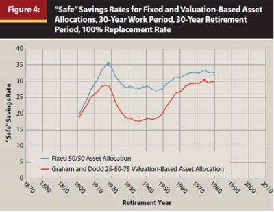
As Pfau (2011a) notes, there is a close correspondence between the MWRs and MSRs for each retirement year. Years when retirees were fortunate to meet their wealth goal with a relatively low savings rate unfortunately tended to find that their retirement period supported a low withdrawal rate. Meanwhile, those unfortunate to retire in years when the required savings rate was quite high, at least tended to find that the withdrawal rate they could have used was also relatively high. Pfau (2011a) suggests, for this reason, to integrate the working and retirement phases to determine the savings rate needed to finance the planned retirement expenditures for rolling 60-year periods from the data, without concern for the implied wealth accumulation and withdrawal rate at the retirement date. That is the “safe” savings rate shown in Figure 4. Comparing the two strategies, the valuation-based strategy offers a lower savings rate at every point in history. The highest of these was 30.4 percent in 1974 for the valuation-based strategy, and 35.4 percent in 1918 for the fixed allocation strategy. These savings rates are much lower than seen in Figure 3 because they exploit the tendency for high withdrawal rates to follow periods supporting low wealth accumulations.
PE5 or PE10
Given the support shown for PE5 in Solow, Kitces, and Locatelli (2011), it is worthwhile to consider how the results change when PE5 is used in place of PE10. For withdrawal rates and PE5, the SAFEMAX is 4.49 percent.
This happened in 1966. The lowest necessary savings rate to meet the wealth target when using PE5 was 77.7 percent, which actually is 1.5 percentage points more than the fixed strategy. The lifetime-based safe savings rate was 33.4 percent. These results are weaker than those using PE10. With PE5, high valuations tend to occur more often during recessions when earnings have declined, suggesting that five years is not long enough to remove the cyclical effects. But these PE5 results do question the overall robustness of the findings.
Changing Allocations in the Wrong Direction
What happens if clients change their asset allocation in the opposite direction of this valuation-based approach? That is, what if clients become enthusiastic for stocks and increase their stock allocation to chase returns after valuations have risen, and then become fearful and lower their stock allocation after valuations have already fallen? There are a number of arbitrary actions clients could consider in this regard. One possibility is the opposite asset allocation strategy of that shown in Figure 1. That is, high valuations result in a 75 percent stock allocation, medium valuations result in 50 percent stocks, and low valuations result in 25 percent stocks. This strategy lowers sustainable withdrawal rates compared with a fixed 50/50 allocation in all years except 1980. The SAFEMAX for this approach was 3.32 percent in 1937, compared with the 3.97 percent SAFEMAX with the fixed allocation. In addition, required savings rates to meet a wealth target were higher in all years except 1997–2008, and lifetime-based savings rates were higher in all years. The safe savings rate increases to 46.12 percent, compared with 35.14 percent for the fixed allocation strategy. Clients clearly would have been harmed historically by having their emotions lead them to deviate in the non-valuation-based direction from their strategic asset allocation.
Conclusions
This article provides favorable evidence based on the historical record for clients to obtain improved retirement planning outcomes (lower savings rates, higher withdrawal rates) using dynamic valuation-based asset allocation strategies. This is illustrated with a specific example comparing a 50/50 fixed allocation strategy to the Graham and Dodd valuation-based strategy with a stock allocation of 25 percent, 50 percent, or 75 percent, determined by the value of PE10 with respect to its rolling median value.
There are caveats though, such as the problem that index funds did not exist until the 1970s, making it quite costly to implement either of these strategies in the past, and taxes or transaction costs have not been incorporated. Implementing the valuation-based allocation strategy does require a certain disposition, as it is a contrarian strategy requiring lower stock allocations when people are most giddy about stocks and higher stock allocations when panic has set in. The fact that the strategies “worked” historically also does not guarantee future success. Nonetheless, this research does propose a potential asset allocation approach for advisers and clients wishing to incorporate valuations into their asset allocation choices, but also wishing to maintain a formal commitment to an asset allocation decision framework that will hopefully help prevent hasty emotion-based decisions.
References
Barber, Brad M., and Terrance Odean. 2000. “Trading Is Hazardous to Your Wealth: The Common Stock Investment Performance of Individual Investors.” Journal of Finance 55, 2 (April): 773–806.
Bengen, William P. 1994. “Determining Withdrawal Rates Using Historical Data.” Journal of Financial Planning 7, 4 (October): 171–180.
Blanchett, David. 2011. “Is Buy and Hold Dead? Exploring the Costs of Tactical Reallocation.” Journal of Financial Planning 24, 2 (February): 54–61.
Campbell, John Y., and Robert J. Shiller. 1998. “Valuation Ratios and the Long-Run Stock Market Outlook.” Journal of Portfolio Management 24, 2 (Winter): 11–26.
Fisher, Kenneth L., and Meir Statman. 2006. “Market Timing in Regression and Reality.” Journal of Financial Research 29, 3 (Fall): 293–304.
Frazzini, Andrea, and Owen A. Lamont. 2008. “Dumb Money: Mutual Fund Flows and the Cross-Section of Stock Returns.” Journal of Financial Economics 88, 2 (May): 299–322.
Graham, Benjamin, and David Dodd. 1940. Security Analysis (The Classic 1940 Second Edition). New York: McGraw-Hill.
Jenkins, David. 1961. How to Profit from Formula Plans in the Stock Market. Larchmont, NY: American Research Council.
Kitces, Michael E. 2008. “Resolving the Paradox—Is the Safe Withdrawal Rate Sometimes Too Safe?” The Kitces Report (May).
Kitces, Michael E. 2009. “Dynamic Asset Allocation and Safe Withdrawal Rates.” The Kitces Report (April).
Pfau, Wade D. 2011a. “Safe Savings Rates: A New Approach to Retirement Planning over the Life Cycle.” Journal of Financial Planning 24, 5 (May): 42–50.
Pfau, Wade D. 2011b. “Can We Predict the Sustainable Withdrawal Rate for New Retirees?” Journal of Financial Planning 24, 8 (August): 40–47.
Pfau, Wade D. 2012. “Long-Term Investors and Valuation-Based Asset Allocation.” Applied Financial Economics, forthcoming.
Ritchlin, Lance. 2011. “William Bengen on Risk, Volatility, and Safe Withdrawal Rates in Today’s Markets.” Journal of Financial Planning 24, 12 (December): 18–20.
Shiller, Robert J. 2000. Irrational Exuberance. 2nd ed. New York: Doubleday.
Shiller, Robert J. 2010. “Irrational Exuberance Revisited.” In Behavioral Finance and Investment Management. Arnold S. Wood, ed. Charlottesville, VA: Research Foundation of the CFA Institute.
Smithers, Andrew, and Stephen Wright. 2000. Valuing Wall Street: Protecting Wealth in Turbulent Markets. New York: McGraw-Hill.
Solow, Kenneth R., Michael E. Kitces, and Sauro Locatelli. 2011. “Improving Risk-Adjusted Returns Using Market-Valuation-Based Tactical Asset Allocation Strategies.” Journal of Financial Planning 24, 12 (December): 38–49.
Stein, Ben, and Phil DeMuth. 2003. Yes, You Can Time the Market. Hoboken, NJ: John Wiley and Sons.
Tomlinson, Joseph A. 2010. “Shiller PEs and Modeling Stock Market Returns.” Advisor Perspectives (January 19).
Tomlinson, Lucille. 1953. Practical Formulas for Successful Investing. New York: Wilfred Funk.