Journal of Financial Planning: September 2013
Executive Summary
- This paper demonstrates how two simple formulas can be used to determine the optimal portfolio withdrawal amount each year during retirement. The first formula, which is called the dynamic formula, determines the withdrawal percentage for a given target probability of success, portfolio equity allocation, expected retirement period, and fees (or alpha). The second approach, which is called the RMD approach, is based on the IRS’ required minimum distribution (RMD) rule. This approach requires only an estimate of the expected retirement period.
- A measure called the “withdrawal efficiency rate” is used to determine the optimal inputs for distribution equations, as well as the relative efficiency of the formula approach.
- Results indicated that life expectancy (median mortality) plus two years is a relatively efficient estimate for the expected retirement period and that 80 percent is a reasonable input for the probability of success.
- Paper equations capture 99.9 percent of the relative efficiency of a far more complex methodology and represent a significant improvement over a static approach. This suggests that while simple, the formulas are nevertheless an incredibly efficient method to implement a dynamic withdrawal strategy for a retiree.
David M. Blanchett, CFP®, CFA, is head of retirement research at Morningstar Investment Management.
Acknowledgments: The author thanks Alexa Auerbach and Michael Finke for helpful edits and comments.
A growing body of research has noted that updating a retirement portfolio withdrawal strategy on a regular basis improves outcomes. Financial planners call this a “dynamic” technique to retirement income, because the portfolio withdrawal amount adapts to ongoing expectations and actual experiences during retirement. This dynamic approach is in contrast to the static approach used in much of the existing literature on sustainable withdrawal rates. The static approach assumes that a retiree selects a withdrawal rate at retirement and subsequently increases the portfolio withdrawal amount to maintain a real level of consumption, regardless of portfolio performance, expected mortality, or the retiree’s changing needs.
While the ability to account for new information makes dynamic withdrawal strategies theoretically superior, many financial planners and engaged retirees may find a dynamic withdrawal strategy difficult or impossible to implement given the sometimes complex software, tools, or processes that are needed to adjust portfolio withdrawal amounts at some regular interval.
This paper introduces two simple equations that can be used to implement an efficient dynamic withdrawal strategy based on different expected time periods, portfolio equity allocations, the likelihood of achieving the goal, and fees (or alpha). There are significant potential benefits to retirees from using this approach, as proxied through a metric termed in this paper as the withdrawal efficiency rate.
Previous Withdrawal Research
The question of how to estimate a safe portfolio withdrawal rate within a retirement income plan is a topic of great debate. Bengen (1994) was one of the first researchers to estimate how much income can be obtained from a portfolio over a retiree’s lifetime (in the absence of annuities). Like most subsequent research, Bengen used an outcomes metric similar to Roy’s (1952) “safety-first rule,” which identifies the optimal portfolio withdrawal amount based on the probability of achieving a goal over a historical time period.
The term “initial withdrawal rate” is commonly used within portfolio withdrawal strategy research to describe the initial percentage withdrawn from the portfolio. This percentage is assumed to increase thereafter by the rate of inflation. For example, an initial portfolio with a $1 million balance and a 4 percent initial withdrawal would allow $40,000 of income (that is, pre-tax consumption depending on the tax status of the account) in the first year. If inflation was 3 percent during the first year, the withdrawal for the second year would be $41,200 ($40,000 x 1.03 = $41,200). This inflation-adjusted amount of income is continually recalculated and withdrawn from the portfolio until it is exhausted. This represents a static approach to portfolio income, because the real income amount is not changed over time.
Although assuming a constant real income during retirement makes a retirement income analysis relatively easy, in reality it is likely a retiree will change the portfolio withdrawal based on the realized performance of the account and the remaining expected retirement period. For example, if portfolio performance is greater than expected, the retiree could increase the portfolio withdrawal amount, but if the portfolio does poorly (worse than originally projected), a retiree may opt to reduce spending to minimize the likelihood of financial ruin. A withdrawal strategy where the portfolio amount is revisited at some frequency throughout retirement to take into account experiences and expectations is known as a dynamic approach.
Milevsky and Huang (2011) noted that following a static approach, like the 4 percent rule, is consistent with life cycle consumption smoothing only under a very limited set of implausible preference parameters. The static approach is unrealistic for any client who can accept some risk of having to reduce consumption late in life. The optimal behavior for a retiree in the face of longevity risk is to consume some amount of income based on survival probabilities and the current likelihood of being able to achieve some level of income, versus blindly withdrawing constant income for life.
Dynamic Strategy Research
Bengen (2001) and Pye (2001) were among the first to comment on dynamic strategies, and since this early research, dynamic withdrawal strategies have become increasingly complex. For example, Guyton (2004) and Guyton and Klinger (2006) used different decision rules to determine when and how to adjust a portfolio withdrawal strategy, such as the capital preservation rule, the prosperity rule, and the withdrawal rule. Stout and Mitchell (2006) developed a model where adjustments to retirement withdrawal rates are based on both portfolio performance and remaining expected mortality.
Blanchett and Frank (2009) used an approach where the portfolio withdrawal amount is determined each year based on the probability of failure of achieving the goal over the remaining distribution period. Their method is similar to Stout and Mitchell (2006), but is more dynamic and allows the user to input more parameters into the ongoing portfolio withdrawal decision.
Milevsky and Robinson (2005) introduced a measure called stochastic present value, which quantifies the amount of reserves needed today to fulfill all future liabilities for a given level of certainty. This metric, often used by actuaries, provides an estimate of safe spending rates without resorting to Monte Carlo simulations.
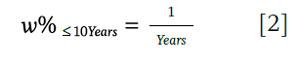
One dynamic strategy that has received increased attention is the so-called RMD approach. A required minimum distribution (RMD) is the minimum amount that a retirement plan account owner must withdraw annually starting with the year that he or she reaches age 70½ or, if later, the year in which he or she retires. Retirees who simply consume their RMDs engage in a dynamic strategy that involves multiplying the account balance by one over the remaining expected retirement period. For example, if the retirement period is expected to be 20 years, the portfolio withdrawal in that year would be 5 percent (1/20 = 5 percent) of the portfolio balance.
Sun and Webb (2012) found that the RMD approach performs better than plausible alternatives, such as spending interest and dividends, consuming a fixed 4 percent of initial wealth, or decumulating over the household’s life expectancy. Blanchett, Kowara, and Chen (2012) also noted the relative efficiency of the RMD approach, primarily because of the method’s simplicity.
Estimating Withdrawal Rates
In theory, the optimal withdrawal from a retiree’s portfolio would be determined each year the way the initial withdrawal amount is determined; namely through a comprehensive analysis of that retiree’s facts and circumstances. These updates would recognize, for example, that if the markets perform better than expected, the portfolio withdrawal could potentially increase over time and vice versa. The concept forms the basis of the approach introduced by Blanchett and Frank (2009) and expanded upon in Blanchett, Kowara, and Chen (2012).
Blanchett et al. (2012) tested different withdrawal strategies with varying levels of dynamic parameters. They found (not surprisingly) that the more dynamic and adaptive a withdrawal strategy is, the better off it makes the retiree. The most efficient withdrawal strategy noted by Blanchett et al. is one they called “mortality updating failure percentage.” This approach directly incorporates the current portfolio value, expected portfolio returns, and the expected mortality of the retiree when determining how much should be withdrawn from a portfolio each year during retirement. This method is termed the dynamic complex (DC) approach for the remainder of the paper.
The key information required to implement the DC approach is a database of the optimal withdrawal percentages for each year given different parameters (for example, different retirement periods, equity allocations, target success rates, fees, etc.). The calculations required to develop (and update) this database are computationally complex and likely impractical for the vast majority of financial planners or engaged retirees to implement in the real world. Therefore, this paper attempts to determine if it is possible to estimate the optimal withdrawal for a given number of parameters.
A number of Monte Carlo simulations were conducted, each consisting of 10,000 runs, where the optimal initial withdrawal rate was solved given different parameters, such as retirement period (Years), equity allocation (Equity%), target probability of success (PoS), and fees (Alpha). Various withdrawal periods were tested (five years to 40 years in five-year increments), portfolio returns (0 percent stocks to 80 percent stocks in 20 percent stock increments), probabilities of success (50 percent to 95 percent in 5 percent increments), and fees –2 percent to +2 percent in 1 percent increments) to better understand the relationship of each variable on the respective initial withdrawal rate.
For each simulation the initial withdrawal rate was the assumed withdrawal from the portfolio in the first year of the retirement period, where that dollar amount was then assumed to be withdrawn in the future, and increased (or potentially decreased) by inflation. The implicit assumption within this model is that the retiree will follow the same real (inflation-adjusted) consumption path over the entire period. In reality, though, it is more reasonable to expect the withdrawal to be updated annually to maintain some level of certainty.
Returns for the simulation were based approximately on Ibbotson Associates’ 2012 capital market assumptions, where the assumed returns for stocks was 10 percent¹ with a standard deviation of 20 percent. The assumed return for bonds was 4 percent with a standard deviation of 7 percent, inflation was assumed to be 2.5 percent, and the correlation between the returns of stocks and bonds was .10. The returns for different portfolio equity allocations are included in Table 1.
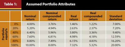
The alpha portion of the analysis enables the reader to more easily adjust the assumed return of a portfolio if his or her capital market assumptions differ from those used for this analysis, as well as incorporating fees. For example, if a financial planner believes the future returns for a 60 percent equity portfolio will be 2 percent lower than the assumed returns for the Monte Carlo simulations, the assumed alpha would be –2 percent. Along these same lines, if a financial planner were to charge 1 percent for his or her services, alpha would be –1 percent.
The Dynamic Formula
After running different types of regressions over different periods, two equations (or models) were created that can be used to approximate the initial portfolio withdrawal percentage over two different periods, for either periods greater than 15 years or less than 15 years. Equation 1 is optimized for retirement periods that are 15 years or greater, where the withdrawal rate is determined given a particular target distribution period (Years), equity allocation (Equity%), target probability of success (PoS), and fees (Alpha). Equation 1 is called the dynamic formula.
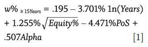
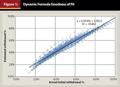
The dynamic formula does a very good job of describing the relationship among these variables and the initial withdrawal rate. The equation yields an R² (coefficient of multiple determination) of 95.48 percent across 1,750 scenarios. The contrasting predictive ability of the dynamic formula compared to the actual withdrawal rates resulting from the Monte Carlo simulations are shown in Figure 1. In terms of the relative differences between the estimated withdrawal rates (equation 1) and the actual withdrawal rates, 46.42 percent of the withdrawal differences are less than .2 percent (in absolute terms), 86.14 percent are less than .5 percent, and only .6 percent of all observatations are above 1.0 percent.
For example, using the dynamic formula, if a planner were to assume a retirement period of 30 years, an equity allocation of 40 percent, a 90 percent probability of success, and an alpha of –1.0 percent (i.e., total fees of 1.0 percent) the estimated withdrawal percentage according to the dynamic formula would be 3.15 percent (the actual value is 3.22 percent). If a planner were to reduce the retirement period from 30 years to 20 years, the withdrawal percentage increases to 4.65 percent (the actual value is 4.62 percent). The formula does a very good job of approximating the withdrawal rate that would be determined through solving a Monte Carlo simulation for the target parameters.
The RMD Approach
For periods shorter than 15 years, using equation 2 is suggested. Equation 2 is called the RMD approach, and it is based on the IRS’ required minimum distribution (RMD) rule. The following variables have been excluded from equation 2 because they do not materially improve the explanatory power of the model: (1) equity allocation (Equity%) (2) target probability of success (PoS) and (3) fees (Alpha).
The R² for the RMD approach over the period (15 years or less) is 95.10 percent, versus 97.65 percent for a more complex four factor model. It is important to note that although the RMD approach results in an estimated withdrawal that is relatively similar to the actual withdrawal for periods of 15 years or less (R² of 95.10 percent), it is materially less useful for periods of 15 years or greater, with an R² of 45.76 percent.
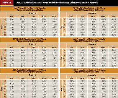
The predictive ability of this two-part model is further demonstrated in Table 2. The left side of Table 2 shows the actual initial withdrawal percentages based on the Monte Carlo simulations for varying retirement periods (in years), equity allocations, probabilities of success, and fees. The right side shows the respective differences in the values determined from the actual Monte Carlo simulations versus using either the dynamic formula or the RMD approach. The model is most accurate for more balanced equity allocations (beween 20 percent and 60 percent) and for more moderate length retirement periods (25 years to 35 years). The purpose of Table 2 is not to necessarily suggest appropriate withdrawal rates. Rather, it demonstrates the effectiveness of the equation by describing the actual results of a Monte Carlo simualtion.
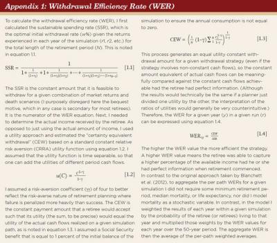
Introducing the Withdrawal Efficiency Rate
This section introduces an approach that can help financial planners determine the optimal inputs for the dynamic formula (retirement periods exceeding 15 years) and the RMD approach (retirement periods less than 15 years), as well as compare the relative efficiency of the optimal parameters against the optimal dynamic approach (DC). This is accomplished using a metric called the “withdrawal efficiency rate” (WER). The WER was originally introduced by Blanchett et al. (2012) and was modified slightly for this paper. Details regarding WER can be found in Appendix 1.
Two key unknowns exist when determining how much a retiree can afford to withdraw from a portfolio: (1) how long the retiree is going to live and (2) the returns the retiree is going to experience. If a retiree knew these two values, he or she could determine the exact amount that could be withdrawn from the portfolio each year (or month) so that the ending value of the account would be exactly $0 on the day he or she (or they) pass away. While it is not possible to know these values in real life, within a simulation framework it is possible to compare the actual income generated by a withdrawal strategy versus the amount of income that could have been withdrawn had the retiree had perfect information. This is the key concept of the WER. WER calculates how well, on average, a given withdrawal strategy compares with what a retiree could have withdrawn if they possessed perfect information on both market returns and the precise time of death.
On average, people prefer to maximize their wealth and achieve certainty (over uncertainty), and the WER metric includes both goals. The WER is calculated by dividing the amount of utility adjusted income received during retirement by the amount of constant income the retiree could have received had he or she had perfect information at the beginning of retirement (that is, they knew the returns that would be experienced and the length of the retirement period). The WER for each run is determined by multiplying the probability of living to that retirement year, subsequent on surviving the previous year, by the WER value for each year of the simulation.
The aggregate WER value for a given strategy is just the average of the WER values for each of the runs of the Monte Carlo simulation. A WER value of 100 percent would imply the portfolio was able to capture all the potential available income over the period and implies the retiree had perfect foresight. Therefore, the goal is to select the strategy with the highest WER value.
Simulations
For the purposes of this paper, the WER metric allows two things to be solved at once. First, it allows financial planners to determine the optimal inputs to use in the dynamic formula and RMD approach (since the inputs that result in the highest WER value would be considered the most efficient). Second, it gives planners the ability to compare the relative efficiency of different retirement income strategies against the DC approach (see the “mortality updating failure percentage” approach in Blanchett et al. (2012)).
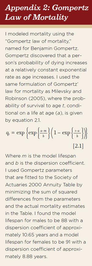
For this analysis, mortality is based on the Society of Actuaries 2000 annuity table. This mortality table is based on those individuals who purchase annuities, and therefore given the adverse selection associated with those individuals who purchase annuities, the life expectancy values are longer than the average person. This table was selected versus using a mortality that reflects average mortality rates, such as the Social Security Administration’s Periodic Life Table, to reflect the assumption that most individuals engaged in determining a withdrawal strategy are likely wealthier and therefore have greater access to health care and are likely to live longer than average.
Independence is assumed when it comes to the life expectancy of the joint spouses, and the retirement period is considered to continue so long as either member of the joint couple is still alive. The Gompertz law of mortality was used to implement mortality and incorporate mortality shocks, as outlined in Appendix 2.
Optimal Input Parameters
Although many financial planners may feel comfortable recommending the appropriate equity allocation given a client’s risk preference and risk capacity, and be able to reasonably estimate the total fees and expected alpha, the retirement period and target probability of success assumptions are more ambiguous, especially because the two are interrelated. They are interrelated because a more conservative retirement period estimate has the same relative effect on the resulting withdrawal rate as a higher probability of success. As a result, both changes would cause the initial withdrawal to decrease.
When thinking about the optimal input parameters, it is important to balance ease of calculation against complexity. For example, the most commonly cited metric when discussing how long someone is going to live is life expectancy. Life expectancy is the median expected mortality for a given individual, where there is a 50 percent chance of dying before that age and a 50 percent chance of dying after it. While it is common to use retirement periods longer than life expectancy in financial plans (for example, 30+ years for a joint couple), this is usually an ambiguous process that is difficult to implement for different clients (for example, a married couple both age 60 versus a single male age 80) while it is relatively easy to estimate life expectancy using a number of free tools online.
The retirement period for this analysis was estimated using a “life expectancy plus” approach, where some number of years was added beyond life expectancy when estimating the assumed length of the retirement period. For example, based the Society of Actuaries 2000 annuity mortality table, the life expectancy for a 65-year-old male is approximately 21 years (versus 24 years for a female and 28 years for a joint couple). Is 21 years the optimal target retirement period when estimating the optimal withdrawal using equations 1 and 2, or would some higher number, say 25 years, be better?
In addition to estimating the optimal retirement period, planners must also estimate the optimal probability of success. The probability of success is effectively the certainty associated with achieving a goal and represents effectively a trade. A higher (lower) probability of success is going to be associated with a lower (higher) amount of consumption during retirement. While selecting a 99 percent probability of success creates a high degree of certainty for a client, it also comes at the cost of less income. Therefore, it’s important to take a more balanced approach when selecting the acceptable probability of success. In other words, planners and their clients “trade” a higher (lower) likelihood of achieving a goal for less (more) income during retirement.
For the purpose of this study, the optimal joint combination of retirement period and probability of success inputs given different scenarios was determined. Retirement periods from life expectancy (plus zero years) to life expectancy plus 10 years, in one-year increments, were tested. For simplicity purposes, the add-on (or life expectancy “plus” value) was assumed to stay the same over the entire retirement duration. Probabilities of success of 99 percent, 95 percent, 90 percent, 80 percent, 65 percent, and 50 percent were tested in equation 1 (note the mortality period is the only variable in equation 2; therefore, it is not affected by the probability of success).
The optimal inputs across a variety of simulations were determined. Males, females, and joint couples (male and female with the same age) from ages 60 to 85 in five-year increments were tested. Mortality shocks also were assumed. These were assumed to be known to the retiree (that is, the retiree is healthier or less healthy than average and can incorporate this information into the planning period).
For simplicity purposes, a portfolio fee was not included, and a 40 percent equity allocation for the scenarios was assumed. Blanchett et al. (2012) noted the WER methodology is relatively insensitive to the equity allocation, therefore only a moderately aggressive portfolio was considered for simplicity purposes.
A target life expectancy plus two years, with an 80 percent target probability of success, was found to be the optimal parameters in the vast majority of simulations. Among the 66 different combinations considered, the average rank for these parameters (where 1 is best and 66 is worst) was 2.07 for the 80 percent probability of success and life expectancy plus two years input parameters. The worst rank of this combination across all 66 different combinations was 7, and the mode (most common rank) was 1. Interestingly, the efficiency of the approach changed very little for different mortality shocks. However, this is likely because the mortality shock is assumed known to the retiree, and therefore can be incorporated into the mortality projections.
Relative Efficiency
The previous section reported results from an analysis to determine the optimal input parameters for the formulas. In this section, the relative efficiency of these inputs is compared against the dynamic formula model.
It was determined previously that a target life expectancy plus two years with an 80 percent target probability of success to be the global optimal parameters for the equations. Because a slightly modified version of the WER equation was used in this paper versus Blanchett et al. (2012), new optimal parameters for the DC approach were estimated. The same life expectancy plus methodology were used to estimate the retirement distribution period, which was similar to the formula approaches, where life expectancy plus zero to 10 years in one-year increments and target probabilities of success of 99 percent, 95 percent, 90 percent, 80 percent, 65 percent, and 50 percent were considered. This retirement period approach is slightly different than the approach taken by Blanchett et al. (2012) who used a mortality-based probability approach, but the life expectancy plus method actually results in higher WER values, on average.
The same simulations used to determine the inputs for the equation models were solved. Results show that the optimal mortality and probability of success inputs for the DC approach vary by simulation, but are generally life expectancy plus three years with an 80 percent probability of success. Among the 36 different combinations tested across the 54 scenarios, the average rank was 2.14, with the worst rank being 8. These input parameters are very similar to the inputs for the formulas, with the difference being the formulas use life expectancy plus two years, while the DC approach is life expectancy plus three years.
Also ran were simulations assuming a static withdrawal approach where the initial portfolio withdrawal was based on the same portfolio withdrawal percentage in the DC model. Within the static approach, though, the subsequent withdrawal was only the original withdrawal increased (or decreased) by inflation (deflation) without regard to the actual growth of the account.
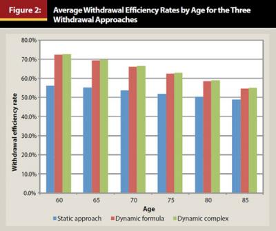
The average WER values for each age considered in the analysis are included in Figure 2. Both the dynamic formula and the DC approach were significantly more efficient than the static withdrawal approach, although the potential increase in efficiency declined for shorter expected retirement periods (that is, older retirees). WER values for the dynamic formula and RMD approaches captured 99.89 percent of the WER values of the DC model, on average.
Spreadsheet Implementation
While the equations introduced in this paper are considerably easier to use than dynamic approaches noted in past research, especially in terms of allowing the user to apply different inputs, these approaches may still be difficult for some financial planners or engaged retirees to implement. Therefore, an Excel spreadsheet has been developed and uploaded for public use (www.DavidMBlanchett.com/tools). This spreadsheet is not meant to be a substitute for a personalized financial plan, but it should provide financial planners (or other users) with a resource to better estimate the appropriate withdrawal rate from a portfolio given a variety of inputs.
Conclusions
There is a growing body of literature noting the potential benefits of a dynamic withdrawal amount (or rate) from a portfolio in retirement. Unfortunately, many of these strategies require complex rules or databases that the average financial planner or engaged retiree may be unable to follow. This paper introduced two formulas to simplify the optimal withdrawal amount calculation. The first equation, called the dynamic formula, works for periods 15 years or greater and can be used to determine a withdrawal rate given a retirement period, equity allocation, target probability of success, and alpha (or portfolio fee). The second formula, which is referred to as the RMD approach, is based on the IRS’ required minimum distribution (RMD) rule. The RMD approach works well for periods less than 15 years and only requires a client’s retirement period as a single input.
Additionally, a method called the “withdrawal efficiency rate” was presented to estimate the optimal inputs into the equations, as well as to determine the potential efficiency loss from implementing this formula approach versus a complex dynamic strategy. It was determined that life expectancy (median mortality) plus two years is a relatively efficient estimate for the expected retirement period and that 80 percent is a reasonable input for the probability of success. A decrease in efficiency of only 0.1 percent versus a considerably more complex dynamic withdrawal approach was noted. Therefore, while simple, these formulas appear to represent an efficient method to implement a dynamic withdrawal strategy for a retiree.
Endnote
- Note that this is the arithmetic average return for stocks, not the compounded (or geometric) return that would be experienced by an investor over an entire investment period. The actual return is reduced by “variance drain,” which can be approximated by subtracting half the variance (which is the standard deviation squared) from the expected arithmetic return. Given an arithmetic return of 10 percent and a standard deviation of 20 percent, the compounded (geometric) return for stocks would be approximately 8 percent.
References
Bengen, William P. 1994. “Determining Withdrawal Rates Using Historical Data.” Journal of Financial Planning 7 (4): 171–180.
Bengen, William P. 2001. “Conserving Client Portfolios During Retirement, Part IV.” Journal of Financial Planning 14 (5): 110–119.
Blanchett, David M., and Larry R. Frank Sr. 2009. “A Dynamic and Adaptive Approach to Distribution Planning and Monitoring.” Journal of Financial Planning 22 (4): 52–66.
Blanchett, David, Maciej Kowara, and Peng Chen. 2012. “Optimal Withdrawal Strategy for Retirement-Income Portfolios.” Retirement Management Journal 2 (3): 7–20.
Guyton, Jonathan T. 2004. “Decision Rules and Portfolio Management for Retirees: Is the ‘Safe’ Initial Withdrawal Rate Too Safe?” Journal of Financial Planning 17 (10): 54–62.
Guyton, Jonathan T., and William J. Klinger. 2006. “Decision Rules and Maximum Initial Withdrawal Rates.” Journal of Financial Planning 19 (3): 48–58.
Milevsky, Moshe A., and Chris Robinson. 2005. “A Sustainable Spending Rate without Simulation.” Financial Analysts Journal 61 (6): 89–100.
Milevsky, Moshe A., and Huaxiong Huang. 2011. “Spending Retirement on Planet Vulcan: The Impact of Longevity Risk Aversion on Optimal Withdrawal Rates.” Financial Analysts Journal 67 (2): 45–58.
Pye, Gordon B. 2001. “Adjusting Withdrawal Rates for Taxes and Expenses.” Journal of Financial Planning 14 (4): 126–136.
Roy, Andrew. D. 1952. “Safety First and the Holding of Assets.” Econometrica: Journal of the Econometric Society 20 (3): 431–449.
Stout, R. Gene, and John B. Mitchell. 2006. “Dynamic Retirement Withdrawal Planning.” Financial Services Review 15 (2): 117–131.
Sun, Wei, and Anthony Webb. 2012. “Should Households Base Asset Decumulation Strategies on Required Minimum Distribution Tables?” Center for Retirement Research at Boston College Working Paper. crr.bc.edu/wp-content/uploads/2012/04/wp_2012-10-508.pdf.
Citation
Blanchett, David M. 2013. “Simple Formulas to Implement Complex Withdrawal Strategies.” Journal of Financial Planning 26 (9): 40–48.