Journal of Financial Planning: March 2014
David W. Johnson, Ph.D., is an associate professor of finance at the University of Wisconsin–Superior and holds a doctorate in finance from the University of Tennessee. Email David Johnson.
Zamira S. Simkins, Ph.D., is an assistant professor of economics at the University of Wisconsin–Superior and holds a doctorate in economics from American University. Email Zamira Simkins.
Executive Summary
- This paper assesses the current and future challenges facing retirees, demonstrates how a reverse mortgage can be used to provide a supplemental source of retirement income, and explains the potential impacts current monetary policy and recent changes to the Home Equity Conversion Mortgage (HECM) program may have on the reverse mortgage market.
- Nearly 80 million baby boomers are expected to retire over the next 18 years. Unfortunately, the recent recession has eroded their retirement portfolio values, increasing retirees’ dependence on Social Security. The long-term solvency of the Social Security system, however, is uncertain. Thus, having alternative sources of retirement income is important. Reverse mortgages are one possible alternative.
- The recent housing market crash has negatively impacted the reverse mortgage market by reducing home values; however, current expansionary monetary policies may create new opportunities. Concerns over the fiscal soundness of the HECM program have necessitated changes to the program requirements that went into effect September 30, 2013. The implications of these changes and monetary policy effects on the reverse mortgage market are discussed in this paper.
The term “baby boomer” refers to a generation of Americans born between 1946 and 1964. The first cohort of baby boomers began retiring in 2011 (2008 for early retirees). The last cohort is expected to retire in 2031. The baby boomer generation represents one of the largest retirement groups in U.S. history. As of December 2011, there were 76.5 million baby boomers, or about 25 percent of the current U.S. population (U.S. Census Bureau 2011a).
Meanwhile, the U.S. birth rate has steadily declined from approximately 25 live births per 1,000 people per year in the 1950s to the current rate of 14 births per 1,000 people. During the same period, life expectancy increased from an average of 67 years to the current average of 77 years, with women effectively breaking the 80-year life expectancy mark in 2005, according to World Development Indicators 2012. As a result, the U.S. dependency ratio is increasing, adding pressure to an already fragile Social Security system.
Although Americans are living longer, they are not necessarily living in better health. As a result, the need for long-term care and health care is also increasing. According to the Employee Benefit Research Institute (2012), a typical 65-year-old couple will need an estimated $305,000 to cover out-of-pocket health care costs over their lifetime. Most people, however, tend to underestimate their life expectancy, save less than they should, and fail to factor in how much health care could cost in retirement. The Employee Benefit Research Institute’s 2012 Retirement Confidence Survey found that 56 percent of workers have not taken the time to calculate how much money they will need to live comfortably in retirement.
Only 33 percent of all private sector workers currently have a defined benefit plan that provides retirement benefits beyond Social Security (Munnell, Haverstick, and Soto 2007). The average monthly Social Security benefit, however, is only $1,230, according to the Social Security Administration. In addition, nearly 60 percent of workers have less than $25,000 in savings and investments, excluding the value of their home (Weber and Chang 2006). Even retirees who planned, saved, and invested for retirement were negatively impacted by the recent recession. A significant number of retirees rely on Social Security as their primary source of retirement income and on Medicare as their main source of health insurance. Specifically, about two-thirds of age-related Social Security beneficiaries receive one-half or more of their income from Social Security, while Social Security is the only source of income for approximately 20 percent to 24 percent of the elderly (Tacchino 2003; Center on Budget and Policy Priorities 2012). The financial future of these programs, however, is uncertain.
Currently, the U.S. Social Security system is largely a pay-as-you-go program, with workers paying taxes that fund the benefits of current beneficiaries. The majority of baby boomers are currently paying into the system. According to the Social Security Administration1, in 2011 there were 28 retirees per 100 tax-paying workers. By 2030, this ratio is expected to increase to 40, and by 2090 to 45. Factoring in young dependents portrays an even gloomier picture, with the overall dependency ratio equal to 35 beneficiaries per 100 workers in 2011, 47 in 2030, and 52 by 2090. Currently, the overall ratio translates into three workers for each dependent. By 2030 and beyond, the ratio will deteriorate to 2:1. In comparison, in the 1960s, there were more than five workers for each beneficiary (Reznik, Shoffner, and Weaver 2005).
These demographic trends raise concerns about the long-term solvency of the U.S. Social Security system. The country’s future implicit liabilities, such as spending on Social Security and Medicare, are expected to increase from the current level of 10 percent of U.S. gross domestic product (GDP) to more than 16 percent of GDP in 2037, and will reach 25 percent of GDP by 2085, according to the Congressional Budget Office’s 2012 long-term budget outlook. Forecasts suggest that by 2021, the Social Security’s Old-Age, Survivors, and Disability Insurance (OASDI) program costs will exceed its total income. By 2033, the program will exhaust all of its assets. After that, taxes paid by workers will cover only 73 percent to 75 percent of the program’s expenditures, according to the Social Security Administration.
To keep the Social Security system financially solvent, several policy reforms have been proposed, including reducing retirement benefits, increasing the retirement age, raising taxes, offering incentives to delay retirement, and encouraging individual retirement savings. Regardless of the policy track the government pursues, it is clear that future retirees should plan on having alternative sources of retirement income to support them in their golden years.
Reverse Mortgage as a Retirement Alternative
Having alternative sources of retirement income is critical for those who are currently retired, those retiring in the near future, and those planning to retire in the next 30 to 40 years. One alternative available to many Americans is a reverse mortgage. Surveys show that Americans tend to store more than two-thirds of their wealth in their homes, which implies that housing, as a retirement asset, will grow in importance in the future (Society of Actuaries 2011). This alternative may be particularly attractive to the baby boomer generation who have high homeownership rates and have conserved their home equity (Poterba, Venti, and Wise 2011).
According to the U.S. Census Bureau (2011b), in 2011, the homeownership rate was more than 70 percent among younger baby boomers and more than 80 percent among older, retiring baby boomers. With the first wave of baby boomers beginning to retire at a rate of more than 10,000 retirees per day, a trend expected to continue for the next 18 years2, the demand for reverse mortgages should increase. The recent housing market crash has had a negative impact on the reverse mortgage market, but the current expansionary monetary policy may create new opportunities. In the long term, reverse mortgages likely will become a significantly more important part of retirement planning.
The HECM Program
A reverse mortgage is a loan that enables senior homeowners to borrow against the equity in their home without having to make monthly mortgage payments. Owners retain title to the home and they may live in the home as long as they choose. As of January 13, 2014, lenders are required to assess the financial condition of prospective borrowers to determine if their income is sufficient to pay future property taxes and insurance. If income is determined to be insufficient, the lender will be authorized to set aside funds from the reverse mortgage to pay those obligations.
Private lenders first introduced the reverse mortgage concept in the 1950s, but it did not gain popularity until 1987 when Congress authorized the Department of Housing and Urban Development to administer a new reverse mortgage program called the Home Equity Conversion Mortgage (HECM) Insurance Demonstration. The HECM is a reverse mortgage insured by FHA, a branch of the U.S. Department of Housing and Urban Development (HUD). Currently, HECMs account for nearly all reverse mortgages issued in the United States, according to the National Reverse Mortgage Lenders Association.
Eligibility for a reverse mortgage requires that loan applicants own their home. The home must be their primary residence, and the youngest borrower must be at least 62 years old. The lender places a first lien on the property, but the homeowner retains title to the home and is liable for insurance, taxes, and property maintenance. Under federal rules, to obtain an HECM loan, consumers must first undergo financial counseling with an independent third party approved by HUD.
The amount a borrower is eligible to receive depends on the age of the youngest borrower, property value, current interest rates, and any existing mortgages or liens that must be settled at closing (existing mortgages can be paid with proceeds from the reverse mortgage). The older the homeowner, the more valuable their home, and the lower the interest rate, the greater the benefit they are eligible to receive. Proceeds are tax free and there are no restrictions on how the money may be spent.
The ability to obtain a reverse mortgage is not dependent on credit history, income level, or health; however, Section 203(b) of the National Housing Act does impose limits on how much can be borrowed. These national lending limits are set by HUD and may be adjusted periodically. In 2013, the lending limit was $625,500. Lending limits do not mean homes of greater value are ineligible for the HECM program; instead, lending rules limit the amount of home value that can be used to calculate a borrower’s eligible loan amount.
Unlike a traditional mortgage that has a maturity and requires monthly payments, a reverse mortgage does not require monthly payments and does not come due until the last surviving borrower permanently moves out of the home. If the home is sold, if the borrowers die, or if the home is not occupied as a principal residence for more than one year, the reverse mortgage comes due and must be repaid. Similar to a traditional mortgage, the borrowers retain title to the property and can sell, refinance, or pay off the loan at any time without a prepayment penalty. They can also leave their home to their heirs. If the selling price exceeds the amount due, the borrowers or heirs keep the excess proceeds.
Mortgage insurance, paid by the borrower, is unique to the HECM product. Mortgage insurance guarantees the homeowner will continue to receive benefits no matter what happens to the lender, and it guarantees they will never owe more than the value of the home. An HECM is a non-recourse loan. This means the borrower, or his or her estate, will never owe more than the loan balance or the value of the property, whichever is less. No assets other than the home must be used to repay the debt. HECM borrowers may receive mortgage proceeds according to six basic payment plans:
Tenure: equal monthly payments for as long as one borrower resides in the home as his or her principal residence.
Term: equal monthly payments for a fixed number of months selected by the borrower.
Line of credit: unscheduled payments or installments at times and in amounts of the borrower’s choosing, until the line of credit is exhausted. A unique feature of the HECM line of credit is that it grows over time, providing a hedge against rising costs.
Modified tenure: a line of credit and equal tenure monthly payments.
Modified term: a line of credit and equal monthly payments for a fixed number of months selected by the borrower.
Lump sum: all proceeds are paid in a single amount at closing, with the maximum allowable disbursement at loan closing or during the first year of the loan being restricted to 60 percent of the eligible benefit or the mandatory obligations plus 10 percent of the benefit. Mandatory obligations are defined as, “Fees and charges incurred in connection with the origination of the HECM that are paid at closing….”3 If the initial disbursement exceeds the 60 percent threshold, a higher upfront mortgage insurance premium (MIP) is assessed on the loan.
Many of an HECM’s costs are similar to those found in a traditional forward mortgage. Upfront fees, paid at closing, include:
- Origination fee to the lender equal to 2 percent of the initial $200,000 of home value plus 1 percent on the balance thereafter with a cap of $6,000. If this amount is less than $2,500, the lender is allowed to charge $2,500. HECM origination fees may be negotiable.
- Third-party fees, such as appraisal, title search, and recording fees.
- If less than 60 percent of available funds are accessed in the first year of the HECM, the upfront mortgage insurance premium (MIP) is equal to 0.50 percent of the home value or the 203(b) limit, whichever is less. If greater than 60 percent of available funds are withdrawn the first year, the upfront MIP is 2.5 percent.
All of these fees may be financed into the loan to create no out-of-pocket costs. When upfront fees are financed into the loan, the borrower will begin with a positive loan balance and interest will begin to accrue on the balance immediately after closing. Fees that accrue over the life of the loan include MIP equal to 1.25 percent of the outstanding loan balance; interest expense, calculated on the outstanding loan balance; and a servicing fee, generally $30 to $35 per month (servicing fees may be negotiable).
The MIP fee of 1.25 percent is added to the note’s interest rate and accrues alongside interest expense each month, based on the loan’s outstanding balance. The lender’s servicing fee is also added to the loan balance each month, as it is incurred. On a typical forward mortgage, the servicing fee is added to the interest rate, effectively raising the interest rate and making the loan’s costs less transparent to the borrower. FHA requires lenders to set aside or reserve, at closing, an amount equal to the present value of future servicing fees, assuming the borrower lives to age 100. Unlike other upfront costs that represent an actual cash outflow and are usually financed into the loan, the servicing set-aside is not added to the principal balance of the loan and does not represent a cash outflow. The set-aside represents an amount of home equity the borrower cannot access via the reverse mortgage, thus reducing the amount of available loan proceeds.
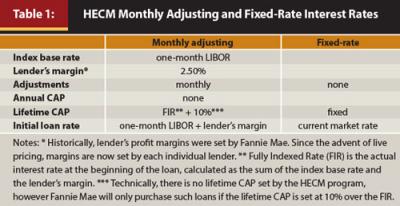
Two HECM loans are currently available to consumers: a fixed-rate and an adjustable-rate loan. Table 1 depicts HECM interest rate information for each loan type. Prior to 2008, as the primary supplier of money loaned in the HECM program, Fannie Mae set the lender’s margins. Because margins and the index base rate were the same for each lender, HECM interest rates were identical for all lenders. Currently, there may be significant differences in margins from lender to lender.
HECM Cash Flows
To illustrate the costs and benefits of a reverse mortgage, the case of a 75-year-old borrower is examined. Assume the borrower resides in a home that is free of any liens and appraised at $400,000. The borrower’s maximum claim amount is equal to the lesser of the appraised value or 203(b) limit of $625,500. In this case, the maximum claim amount is $400,000.
The maximum amount a borrower is eligible to receive from a reverse mortgage is called the principal limit. The principal limit, at origination, is based on the age of the youngest borrower, the maximum claim amount, and the loans expected rate (ER). The expected rate for the HECM LIBOR monthly adjustable loan is the sum of the lender’s margin and the 10-year swap rate. It should be noted that the expected rate differs from the loan interest rate applied to the outstanding loan balance each period. Whereas the loan rate (LR) is used to calculate accrued interest each period and future principal limits, the ER is used for calculating the initial principal limit, servicing set-asides, and payment plans. Because these cash flows occur throughout the life of the loan, they are computed using the longer term, 10-year swap interest rate, as it represents a forecast of future short-term rates likely to be realized over the life of the loan.
The initial principal limit is calculated as the product of the maximum claim amount and a principal limit factor (PLF). The PLF is determined by the age of the youngest borrower and the loan’s expected interest rate. The factors used for calculating principal limits can be accessed at www.hudclips.org. The PLF determines how much of the available home equity (or 203(b) limit if binding) the borrower may access. The factor increases with age and decreases with the loan’s expected interest rate. Based on October 22, 2013, interest rate data and the new principal limit factor tables that went into effect on September 30, 2013, the borrower’s current expected rate is 5.25 percent and the principal limit factor is 0.563. Hence, the initial principal limit is equal to $225,200, which is calculated as:
Expected rate = lender margin + 10-year swap rate = 2.5% + 2.75% = 5.25%
Loan rate = index base rate + lender margin = 0.17% + 2.50% = 2.67%
Principal limit factor (age 75, expected rate 5.25%) = 0.563
Maximum claim amount = $400,000
Initial principal limit = $400,000 * 0.563 = $225,200
Initial MIP = (.005) * maximum claim amount of $400,000 = $2,000To determine the maximum amount of funds this borrower is eligible to receive, a net principal limit is calculated by subtracting any initial payments made to or on behalf of the borrower (for example, initial MIP, origination fees, closing costs, liens, cash payments to the borrower, and funds set aside for monthly servicing fees). It is assumed the borrower does not require any cash payments at closing, but would like to finance the upfront 0.5 percent MIP, origination fees, and all closing costs, which are estimated to equal $2,322.
Origination fee = (.02) * $200,000 + (.01)* $200,000 = $6,000
Closing costs = $2,322
The servicing set-aside is the present value of monthly service fees to age 100. The discount rate (DR) used is the sum of the loan’s expected rate and monthly MIP of 1.25 percent. The calculation assumes payments are made at the beginning of each month. It is assumed the borrower’s loan carries a $30 monthly servicing fee, so the required set-aside is equal to $4,466.98. Recall, the set-aside is not an actual cash outflow; rather it reduces the amount of equity the borrower is able to access. The calculation is:
N = 25 years * 12 = 300 months
Discount rate = (5.25% + 1.25%) / 12 = 0.5417% per month
PV = $4,466.98
Deducting the borrower’s upfront cash requirements (initial MIP, origination fee, closing costs, and servicing set-aside) yields a net principal limit of $210,411.02:
Initial principal limit $225,200.00
Less: MIP – $2,000.00
Origination fee –$6,000.00
Closing costs –$2,322.00
Servicing set-aside –$4,466.98
________________________________
Net principal limit 210,411.02
The borrower can select any of the six payment plans previously discussed as long as the payments plus accrued interest, monthly MIP, and servicing set-asides do not exceed the principal limit. Two of the most common payment options are provided below.
Term option. Payments for the term option are calculated as an annuity having a present value equal to the net principal limit. If the borrower wishes to receive monthly payments for 10 years, then he/she would be eligible to receive $2,376.34 per month:
PV = $210,411.02
N = 10 years * 12 = 120 months
DR = (5.25% + 1.25%) / 12 = 0. 5417% per month
PMT (due) = $2,376.34
Similar calculations yield a monthly payment of $2,944.18 for a 90-month term and $1,823.08 for a 180-month term; in effect, the longer the term selected by the borrower, the lower the monthly payment. Because the loan itself carries a variable rate, it is possible for the actual loan balance to exceed the borrower’s net principal limit before the selected term expires. However, payments continue until the end of the selected term, as initially calculated. The borrower is not required to pay off the loan at the end of the term, nor is he or she required to move at the end of the term. However, interest will continue to accrue on the loan balance until the loan is repaid.
Tenure option. The tenure plan calculates monthly payments as if the borrower will reach age 100. For this 75-year-old borrower, the payment is calculated as a 25-year annuity, with a present value equal to the initial principal limit, or $1,413.11 per month. As shown below, regardless of the actual loan balance, payments continue indefinitely, as long as the borrower is living in the property.
PV = $210,411.02
N = 25 years * 12 = 300 months
DR = (5.25% + 1.25%) / 12 = 0.5417% per month
PMT (due) = $1,413.11
Current Monetary Policy and the Reverse Mortgage Market
Since 2007, the Federal Reserve has been conducting an expansionary monetary policy that created a low interest rate environment. As a result, most retirees, with their short-term, low-risk portfolios, have realized very small returns on their investments. The upside of this environment is that the housing market and home values have started to rebound, according to the S&P/Case-Shiller U.S. National Home Price Index. This section discusses the challenges and opportunities facing the reverse mortgage market created by these expansionary monetary policies.
In the summer of 2006, the U.S. financial system began exhibiting liquidity problems. In an August 10, 2007, press release, the Federal Reserve announced that it was “… providing liquidity to facilitate the orderly functioning of financial markets …because of dislocations in money and credit markets."
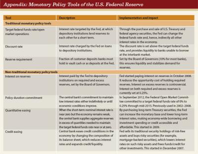
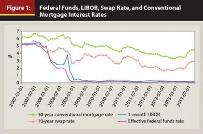
The Fed responded to the liquidity, financial, and economic crises by conducting an unprecedented expansionary monetary policy. Initially, the Fed lowered the discount rate. This was followed by a series of reductions in the federal funds rate (Figure 1). By December 2007, the Fed turned to unconventional monetary policy tools, including credit easing, quantitative easing, policy duration commitment, and payment of interest on reserves (see the appendix for details).
Between 2007 and 2009, the Fed more than doubled the size of its balance sheet and changed its composition by purchasing risky assets from troubled financial institutions, in contrast to the historical norm of acquiring only Treasury securities. In an unprecedented move, the Fed also lent to non-depository institutions. As a result of this expansionary monetary policy, the monetary base nearly quadrupled between January 2007 and April 2013 (Figure 2).
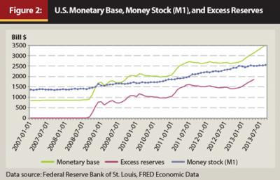
Nevertheless, the liquidity problem persisted. For the first time in U.S. history, the money stock (M1) fell short of the monetary base. The money multiplier process no longer seemed to be working. Between January 2007 and May 2013, commercial banks increased their holdings of excess reserves, or funds they normally loan out, from $1.5 billion to $1.9 trillion, according to Federal Reserve Bank of St. Louis’s Federal Reserve Economic Data, or FRED. This behavior of commercial banks may be explained by their fear of loan defaults and increased risk aversion, or it may be because of the Fed paying interest on all reserves at a rate above the federal funds rate (Simkins 2012).
Persistent liquidity problems pushed the Fed to continue its extraordinary expansionary monetary policy. In September 2012, the Fed announced that it would launch a third round of quantitative easing, injecting even more liquid reserves into apprehensive financial institutions. The Fed committed to keep the federal funds rate within a 0.0 to 0.25 percent target range through mid-2015 to keep short-term interest rates low. Also, the Fed continued its “Operation Twist” program through the end of 2012, under which the Fed sold its short-term Treasury security holdings and bought long-term Treasury securities to keep long-term interest rates low. After the Fed ran out of short-term securities to sell, it continued to purchase long-term securities to maintain low long-term interest rates.
The downfall of the Fed’s expansionary monetary policy is that savers, particularly those saving for retirement, have not seen any significant returns on their savings. However, low interest rates may benefit those considering a reverse mortgage, because LIBOR rates are positively correlated with the federal funds rate, both of which are at a historically low level. Further, the Fed’s long-term interest rate policy has pushed the 10-year swap rate below 3 percent, increasing the monthly benefits received from a reverse mortgage (Figure 1).
The interdependence between the traditional mortgage market and the reverse mortgage market is clear: lower interest rates on traditional mortgages stimulate demand for real estate, resulting in higher home values, which increases the benefits and appeal of a reverse mortgage. If the Fed maintains its commitment to keep interest rates low, the LIBOR, 10-year swap rate, and conventional mortgage rates are likely to remain low. Provided that liquidity conditions improve, current monetary policy has the potential to create favorable conditions for the reverse mortgage market. Until banks increase lending, however, home value appreciation and demand for reverse mortgages will remain sluggish. Ironically, the Fed’s policy of paying interest on excess reserves may have created a disincentive for bank lending. Eliminating the interest paid on excess reserves will not reduce banks’ fear of defaults; however, it will increase the opportunity cost of not lending and may help further stimulate the housing market.
Conclusion
Current and future retirees face a series of challenges that will have a significant impact on their life in retirement. The recent recession negatively affected the value of their investment portfolios and the bursting of the housing bubble diminished the value of their homes. The aging of the baby boomer generation, increased life expectancy, and deteriorating dependency ratios are putting upward pressure on the government’s implicit liabilities and debt. Reliance on Social Security as a primary source of retirement income is no longer a practical solution because of the uncertainty surrounding the solvency of the OASDI program. Furthermore, lack of planning and unrealistic expectations about future costs of basic health care and long-term care will place many retirees in an untenable financial position. Therefore, identifying and using alternative sources of retirement income has become critical for current and future retirees.
Given these challenges and the current interest rate environment, the demand for reverse mortgages likely will increase. In recent years, however, the demand for reverse mortgages has declined. According to HUD, 54,822 reverse mortgage loans were originated in 2012 in contrast with the 114,692 loans originated in 2009. Due to the tremendous amount of equity lost by homeowners during the recent housing crisis, reverse mortgages may not be an attractive alternative at this time. In the long-term, however, this alternative will become a significantly more important part of retirement planning. For growth in the reverse mortgage market to occur, home values must rebound. The Fed, through its expansionary monetary policy, has the potential to stimulate growth in the housing market. To date, however, the Fed’s policies have not had the desired impact on bank lending.
The demand for reverse mortgages also is expected to be affected in the short term by recent changes to the HECM program requirements. These changes were initiated due to concerns over the increased risk of losses and the fiscal soundness of the HECM program. The changes included limitations on the amounts that can be drawn in the first year, the option to receive a smaller one-time single lump sum disbursement, as well as changes to the mortgage insurance premium, the principal limit factor tables, and requiring a financial assessment of borrowers’ ability to pay future property taxes and insurance obligations. The changes to the principal limit factors and limitations on the initial draw resulted in reduced benefits to reverse mortgage borrowers. Based on the case study presented in this paper, the reduction in benefit resulting from the new HECM regulations is 13.8 percent. Therefore, the latest HECM program changes may initially have a small, negative effect on the demand for reverse mortgages. However, because the changes were made to bolster the financial stability of the HECM program, they are expected to produce a positive effect on the reverse mortgage market in the long term.
Historically, many seniors and financial planning professionals have viewed reverse mortgages negatively and considered their use only as a last resort. However, the three legs of the traditional retirement “stool” (Social Security benefits, pensions, and personal savings) have been considerably weakened by the factors described in this paper. Current and future retirees need to re-examine their views and consider including a reverse mortgage as a part of their retirement plan.
Endnotes
See “The 2012 Annual Report of the Board of Trustees of the Federal Old-Age and Survivors Insurance and Federal Disability Insurance Trust Funds” at www.ssa.gov/oact/tr/2012.
See the 2009 Congressional Budget Office paper “Will the Demand for Assets Fall When the Baby Boomers Retire?” at www.cbo.gov/publication/41220.
See “Home Equity Conversion Mortgage Program’s Mandatory Obligations, Life Expectancy Set-Aside Calculation, and Purchase Transactions,” HUD 2013 Mortgagee letter, document number 13-33 at www.hud.gov.
References
Center on Budget and Policy Priorities. 2012. “Policy Basics: Top 10 Facts about Social Security.” www.cbpp.org/cms/index.cfm?fa=view&id=3261.
Munnell, Alicia, Kelly Haverstick, and Mauricio Soto. 2007. “Why Have Defined Benefit Plans Survived in the Public Sector?” Center for Retirement Research at Boston College, State and Local Pension Plans Working Paper #2. http://crr.bc.edu/wp-content/uploads/2007/12/slp_2.pdf.
Poterba, James M., Steven F. Venti, and David A. Wise. 2011. “The Drawdown of Personal Retirement Assets.” NBER Working Paper Series, No. 16675. www.nber.org/papers/w16675.
Reznik, Gayle L., Dave Shoffner, and David A. Weaver. 2005/2006. “Coping with the Demographic Challenge: Fewer Children and Living Longer.” Social Security Bulletin. www.ssa.gov/policy/docs/ssb/v66n4/v66n4p37.html.
Simkins, Zamira. 2012. “Interest on Reserves: A Review of the Federal Reserve’s New Monetary Policy Tool.” Presentation at the Wisconsin Economics Association Annual Conference.
Society of Actuaries. 2011. “Process of Planning and Personal Risk Management.”
Tacchino, Kenn B. 2003. “Retirement Planning—The Rest of the Story.” Journal of Financial Service Professionals: 8-12.
U.S. Census Bureau. 2011a. “National Household Population Estimates.” www.census.gov/popest/data/national/asrh/2011/2011-nat-hh.html.
U.S. Census Bureau. 2011b. “Homeownership Rates for the United States, by Age of Householder and Household Type.” www.census.gov/compendia/statab/2012/tables/12s0992.pdf.
Weber, Joseph A., Echo Chang. 2006. “The Reverse Mortgage and Its Ethical Concerns.” Journal of Personal Finance 5 (1): 37-52.
Citation
Johnson, David W., and Zamira S. Simkins. 2014. “Retirement Trends, Current Monetary Policy, and the Reverse Mortgage Market.” Journal of Financial Planning 27 (3): 52–59.