Journal of Financial Planning: July 2016
Wade D. Pfau, Ph.D., CFA, is a professor of retirement income at The American College, principal at McLean Asset Management, and host of the Retirement Researcher website, RetirementResearcher.com.
One of the important and challenging aspects of retirement income planning relates to how taking distributions from an investment portfolio amplifies the impacts of portfolio volatility. Examples showing this sequence-of-returns risk abound, but I will tackle it in a less commonly viewed way.
Monte Carlo simulations can be used to show how the range of money-weighted investment returns gets larger in retirement. This has important implications about the choice for a fixed portfolio return assumption that should be used when creating financial plans within a spreadsheet. Implied investment returns are usually not shown with Monte Carlo simulation output, but they exist under the hood. What is the implied portfolio return that supported a 90 percent chance for success? We have to reverse engineer Monte Carlo simulations to know this. The implied return will be lower than the average returns inputted into Monte Carlo, and I find empirical support for the idea that portfolio return assumptions for the post-retirement period should be more conservative than for the pre-retirement period.
Basics for Choosing a Portfolio Return Assumption
For a lifetime financial plan, the most intuitive way to express a portfolio return assumption is as an inflation-adjusted compounding return. Unfortunately, this is generally not the most common way returns are expressed. It is worth a quick review of the steps needed to arrive at a real compounded return.
I will illustrate this by focusing on the compounded real returns generated historically by a 50/50 asset allocation to the S&P 500 and intermediate-term U.S. government bonds.
For the period from 1926 through 2015, Morningstar data reveals that the S&P 500 enjoyed an average (arithmetic) return of 12 percent, while intermediate-term government bonds earned 5.3 percent. Removing inflation so that the numbers allow for a better understanding of purchasing power growth, the real arithmetic returns fell to 9 percent and 2.3 percent, respectively. For those simulating long-term financial plans, we also have to account for volatility and the lack of symmetry in outcomes for positive and negative returns. We calculate the compounded returns over time to account for this volatility. The S&P 500 compounded real return fell to 6.9 percent, while the compounded real return for the less volatile bonds fell only slightly to 2.2 percent.
I simulated each asset class separately and combined them into a 50/50 portfolio rebalanced annually. For 100,000 Monte Carlo simulations over 30-year periods, the estimated arithmetic real return from the 50/50 portfolio was 5.6 percent, and the standard deviation for returns was 10.8 percent. The compounded real return was 5.1 percent.
There are a number of further adjustments we could and should make, such as incorporating taxes, accounting for the fact that today’s interest rates are much lower than the historical averages, removing the impacts of advisory and investment fees, and considering the possibility of outperformance or underperformance with respect to the underlying market indices. While these are all important considerations, I will focus here specifically on how advisers should adjust their assumptions to account for sequence-of-returns risk.
The Impact of Sequence Risk
Consider three scenarios: an individual investing a lump-sum amount for 30 years, an individual saving a fixed percentage of a constant inflation-adjusted salary at the end of each year over a 30-year accumulation period, and an individual withdrawing the maximum sustainable constant inflation-adjusted amount from a portfolio at the start of each year over a 30-year retirement period.
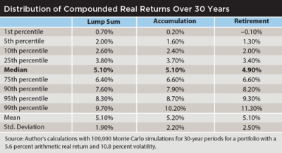
The table provides the distribution of results for the simulations. For the lump-sum investment, the numbers represent the distribution of average compounded returns over the 100,000 30-year periods. For the accumulation phase, the distribution of outcomes is for the internal rate of return when making 30 annual contributions at the end of each year relative to the final accumulated wealth at the end. For the retirement phase, the distribution of results is for the internal rates of return on the portfolio when withdrawing the maximum sustainable amount over a 30-year period with distributions taken at the start of each year.
In all three cases, the median return was close to 5.1 percent, which was the assumed compounded return for the simulations. However, most clients would probably shy away from using this number to develop a financial plan in a spreadsheet, because as the median, the probability that can be achieved is only 50 percent. When choosing a number to plug into a spreadsheet, a conservative client might be more comfortable using something like the return in the 25th percentile, or even the 10th percentile, of the distribution. These numbers would correspond with 75 percent or 90 percent probabilities of success, respectively.
Again, financial planning software does not usually show the implied returns, but this is what the table has provided through a reverse engineering process. With the lump-sum investment, the compounded real return at the 25th percentile is 3.8 percent over 30 years. For an accumulator, the 25th percentile return is 3.7 percent, and it is 3.4 percent for the retiree. At the 10th percentile, realized compounded real returns were 2.6 percent for the lump-sum investment, 2.4 percent for the accumulator, and 2 percent for the retiree. These numbers are naturally lower to provide a greater chance for success, and sequence-of-returns risk contributes to making these numbers even lower for accumulators and retirees than with the lump-sum investment that does not experience sequence risk. The volatility of outcomes increases as we transition from a lump-sum (standard deviation of 1.9 percent) to accumulation (2.2 percent) to retirement (2.5 percent).
Monte Carlo simulations generally present results in terms of a probability for success. Clients may aim for 90 percent success or higher. There is an implied rate of return on the portfolio connected to a given probability of success, though Monte Carlo simulations generally do not express their output in this way. Higher rates of success would be connected with lower portfolio returns, since this return hurdle must be exceeded by the portfolio for the financial plan to be successful. In this discussion, I am tackling Monte Carlo from a different direction—first, using Monte Carlo simulations to get a rate of return for the portfolio, then to simulate a financial plan using a fixed rate of return. Conservative investors will want to work with lower assumed returns, implying a need to save more today.
Clients who are accumulating or spending their assets will have different experiences than implied by a lump-sum investment. Accumulation effectively places greater importance on the returns earned late in one’s career when a given return impacts more years’ worth of contributions. With new contributions each year, the timing of returns matters, as later returns impact more contributions and have a larger impact on final wealth accumulations. This is sequence-of-returns risk as it applies in the accumulation phase. With greater importance placed on a shorter sequence of returns, we should expect a wider distribution of outcomes.
As for retirement, the impacts are even bigger, as sequence risk further amplifies the impact of investment volatility. Retirees experience heightened sequence-of-returns risk when funding a constant spending stream from a volatile portfolio, because portfolio declines imply needing to spend a greater percentage of remaining assets. This digs a hole for the client’s portfolio that can be difficult to overcome. The distribution of internal rates of return during retirement will be even wider because of the heightened importance placed upon the shorter sequence of post-retirement returns. A conservative retiree seeking a return assumption for retirement should use a lower value than pre-retirement.
Sequence risk widens the distribution of outcomes in retirement and retirees also experience less risk capacity. With less time and flexibility to make adjustments to their financial plans, portfolio losses can have a bigger impact on remaining lifetime standards of living once retirees have left the workforce.
This is another reason why clients may want to use different return assumptions pre- and post-retirement. For example, a conservative client might be willing to use the 25th percentile return during accumulation (calibrated to a 75 percent chance for success), but only the 10th percentile during retirement (90 percent success). If the client were comfortable with the arithmetic real return and volatility of 5.6 percent and 10.8 percent, this would suggest using a 3.7 percent compounded real return assumption in the spreadsheet for accumulation and a 2 percent compounded real return assumption in their spreadsheet for retirement, even though the “best guess” about the compounding return they will experience is 5.1 percent.
Because of sequence-of-returns risk, conservative investors may wish to use lower fixed return assumptions than just the compounded return assumed for a lump-sum investment. Sequence-of-returns risk is relevant for both the accumulation and retirement phases. Assumed returns should be lower in both cases. The impact is even greater for retirement. Conservative clients may not want to use the “expected return” for their portfolios when developing lifetime financial plans. This is an important point to remember and to internalize when working in environments that require a return assumption but not an accompanying volatility. ![]()