Journal of Financial Planning: July 2013
Executive Summary
- Much of the research on sustainable retirement withdrawal rates has been based on historical market returns and fairly complex Monte Carlo multivariate scenario analysis using third-party software that is often difficult to customize. A simplified deterministic model, based upon the same Monte Carlo capital market inputs (expected arithmetic return and portfolio volatility) can efficiently provide Monte Carlo type answers to retirement income sustainability.
- The simplified method presented in this paper uses standard deviation for conversion of arithmetic average return to the derived geometric average return for each level of confidence.
- The deterministic model allows financial planners to easily incorporate customized withdrawal or success calculations into their proprietary workflows using a simple spreadsheet program.
- As discussed in this paper, the historical success and more recent failure of the 4 percent rule can be explained by the ratio of the real withdrawal rate to the portfolio arithmetic average return, and also recent market related reductions in the expected geometric average return.
- The deterministic method is especially useful for periodic re-sampling when using an adaptive approach to distribution planning, where the ongoing withdrawal rate is fluid and not constant; this method can further improve the probability of success of a distribution strategy.
Gregory W. Kasten, M.D., CFP®, CPC, AIFA® is founder and CEO of Unified Trust Company. He has published more than 85 papers on financial planning and investment related topics in various financial and business journals and has written two editions of the book Retirement Success. In 2005 he co-wrote the award-winning paper “Post Modern Portfolio Theory” and presented the paper at FPA’s annual conference.
Many financial planning software programs incorporate Monte Carlo probability analysis into a forecasting program to predict retirement income sustainability. As pointed out by several researchers, all too often financial planners and clients do not understand that Monte Carlo results are highly sensitive to even small changes in arithmetic (mean) return, standard deviation, and other risk assumptions (Brayman 2007; Nawrocki 2001).
In fact, a recent study conducting analysis on 10 calculators revealed a wide range of results for a hypothetical retiree, with the lowest giving a sustainability probability of 48 percent and the highest 88 percent (Milevsky and Abaimova 2006). Myriad input problems causing such discrepancies have been well identified in the literature (Turner and Witte 2009). Nawrocki (2001, 93) stated, “Essentially, Monte Carlo simulation is useful only when nothing else will work. It has proved to be useful in academic financial and statistical research, but only when the data or the analytic solution is not available. This is not the case in the investment decisions typically faced by financial planners.”
The main focus of this article is not a criticism of Monte Carlo programs on the market today. Instead, this paper shows that a simplified deterministic model, based upon the same capital market inputs (expected average arithmetic return and portfolio volatility) can efficiently provide Monte Carlo type answers to retirement income sustainability questions. The deterministic model is simpler to use, and because it does not generate a new randomized distribution, the results are the same with each repetitive run.
Building a Deterministic Model
A deterministic model can be built using compounded or geometric average returns. Besides the painful episodes of periodic market declines, volatility is an important factor to consider in portfolio management, and it is necessary to understand why this is the case. The answer lies in the relationship between the geometric average return and the arithmetic average return. The geometric average return is the return that is achieved through reinvestment or compounding, while the arithmetic return is the simple average of the returns. A geometric average return is affected by negative values, and negative values become more likely as the variability—or standard deviation—of the portfolio increases.
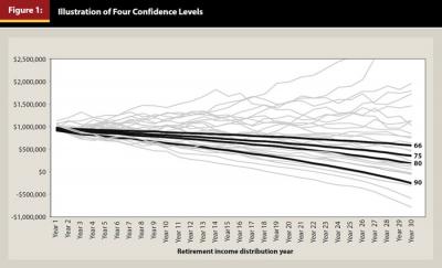
To examine the impact standard deviation has on relating arithmetic average returns to geometric average returns, a Monte Carlo simulator was built to test real (inflation adjusted) arithmetic returns ranging from 0 percent to 10 percent, and portfolio standard deviations ranging from 0 percent to 20 percent. For all tests, inflation was assumed to be a constant 3 percent. The four retirement income confidence levels were targeted at the 66, 75, 80, and 90 percentiles of final year results. Thus, the 80 percentile level of confidence meant that at least 80 percent of all values were greater than that figure. The time horizons studied varied from one to 30 years. To ensure a stable dataset, 50,000 simulations were run for each set of variables. For an illustration of the four confidence level percentile bands, see Figure 1.
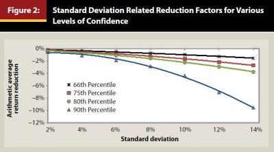
Next, the geometric average return was calculated for each ending portfolio value at the 66, 75, 80, and 90 percentiles. These data were incorporated into a regression analysis model to calculate the geometric average return across all standard deviations for a given level of confidence. A reduction factor was calculated for each level of confidence and for each standard deviation. These reduction factors were then fitted to a best fit polynomial equation across the range of standard deviations for each level of confidence as shown in Figure 2.
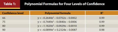
Note that each level of confidence has its own unique conversion formula, as shown in Table 1. The polynomial formulas can be easily programmed into a spreadsheet. After that, the only inputs needed are expected arithmetic average return and portfolio standard deviation, which are, of course, also required for all Monte Carlo applications. These same inputs also would be used for asset allocation mean variance optimizer (MVO) calculations, along with correlations. The polynomial formulas allow conversion from the arithmetic average return to geometric average return, where x is the portfolio standard deviation, and y is the reduction of return from the arithmetic average. Each level of confidence has its own unique impact on geometric average return.
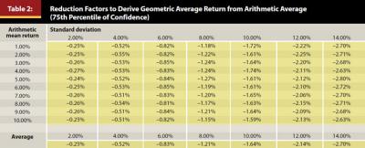
The negative calculated number is added to the arithmetic mean return to give the derived geometric return equivalent at certain higher confidence levels greater than the 50th percentile. For example, in Table 2, using the 75 percentile level of confidence, if the standard deviation is 8 percent, the average deduction from the arithmetic average return is –1.21 percent. Thus, if the real arithmetic average were 4 percent with an 8 percent standard deviation, at the 75 percentile of confidence, the derived real geometric average would be 2.79 percent.
Note that just the opposite calculation occurs for the low confidence 10, 20, 25, and 33 percentiles. In these situations, the negative reduction factor difference is subtracted from the arithmetic average to give the derived geometric average return. For example, using the 25 percentile level of confidence, if the standard deviation is 8 percent, the average deduction from the arithmetic average return is –1.21 percent. Thus, if the real arithmetic average is 4 percent with an 8 percent standard deviation, at the 25 percentile of confidence, the real geometric average would be 5.21 percent. Strictly speaking, the geometric return can never be greater than the arithmetic return, and only equals it when the standard deviation is zero. But the derived geometric average return would be greater than the arithmetic return for determining low confidence (below 50th percentile) results. In this paper, it was assumed that the low confidence 10, 20, 25, and 33 percentile values would not be very useful to most financial planners and therefore they were not included in the remainder of the discussion.
The reduction factor in return per each unit of standard deviation was consistent across a range of arithmetic returns for a given amount of standard deviation. Table 2 demonstrates this consistency across various arithmetic returns for a given amount of standard deviation, in this case from the 75 percentile level of confidence. Similar general consistency for a given amount of standard deviation was found in all four levels of confidence (66, 75, 80, and 90 percentiles).
Using Derived Geometric Average Return to Calculate Sustainable Withdrawal Rates
The derived geometric average return value is very useful for two retirement income calculations. The time period can be any length as desired by the financial planner and client.
The first is to calculate the sustainable withdrawal payout ratio using the PPMT (payment) function in Excel.
The second is to determine how long the portfolio will last for a given withdrawal rate, or in other words, the likelihood of success. This can be calculated using the FV (future value) function in Excel to solve for the number of years when the future value is $0. Because the process is a deterministic method, the answers obtained are precise for a given level of confidence, which leads, in effect, to “yes” or “no” solutions. Unlike Monte Carlo methodologies, each deterministic calculation using the same inputs gives the exact same answer.
To illustrate, it is possible to evaluate capital market data from Bengen’s (1994) original safe withdrawal rate study. In his paper on the sustainability of retirement income, Bengen reported that a 4 percent real (inflation adjusted) withdrawal rate was safe in a variety of market circumstances. Bengen reported that he used Ibbotson Associates’ Stocks, Bonds, Bills, and Inflation (SBBI) data for the years 1926–1992. During this period, stocks provided an arithmetic average return of 10.3 percent, bonds an arithmetic average return of 5.2 percent, and inflation a 3.0 percent rate. Using these data, a 50 percent equity and 50 percent bond portfolio would have a nominal average return of 7.8 percent, a real (net of inflation) return of 4.6 percent, with a standard deviation of 10.2 percent.
Bengen reported that such a portfolio would have survived all periods from 1926–1976. However, this is a very small dataset. When subjected to both Monte Carlo and the deterministic model, it can be seen that such a portfolio is safe most of the time.
The calculations are shown in Figure 3 for the 80 percentile level of confidence with a zero ending dollar balance on the final day of the 30-year retirement period. The capital market data (arithmetic average and standard deviation) are from Bengen’s data.
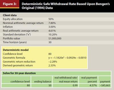
The deterministic analysis indicates Bengen’s (1994) “4 percent rule” gives a high degree of confidence, well in excess of 80 percent. The 80 percentile withdrawal rate in the deterministic model is 4.57 percent. The derived real geometric average return at the 80 percentile confidence level is 2.33 percent. This is sufficiently large enough to generate a real payment of $45,663 at least 80 percent of the time, which is higher than the $40,000 (4 percent) rule. When the same 4 percent withdrawal rate data were run 10,000 times in the Monte Carlo analysis generator, the survivability was 89 percent of all runs.
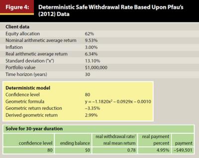
More recently, Pfau (2012) outlined a framework for estimating sustainable withdrawal rates and appropriate asset allocations based on a financial planner’s capital market expectations and asset choices, as well as other inputs about the client’s circumstances. Pfau reported, based upon historical data from the period 1926–2010, that stocks provided an arithmetic average real (post inflation) return of 8.70 percent. Bonds returned an arithmetic average real return of 2.52 percent. Using these data, a 62 percent equity and 38 percent bond portfolio was reported to have an arithmetic average real return of 6.34 percent and a standard deviation of 13.10 percent. When subjected to both Monte Carlo and the deterministic model, it can be seen (Figure 4) that such a portfolio is safe most of the time. In fact, the deterministic model reveals a 4.95 percent withdrawal rate is sustainable in such a portfolio at the 80 percent level of confidence.
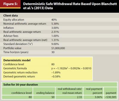
However, several authors have challenged the 4 percent rule on a forward-looking basis (Athavale and Goebel 2011; Blanchett, Finke, and Pfau 2013). In a low interest rate environment, the authors question what withdrawal rate is sustainable. In addition, the Blanchett et al. paper includes the impact of 1 percent advisory fees on portfolio returns. These concerns can be partially explained by examining the ratio of the real withdrawal rate to the expected real arithmetic portfolio return, and also the derived real geometric return. Recall in Bengen’s (1994) original study the ratio of the real withdrawal rate to the real arithmetic return was 0.99, and in Pfau’s (2012) study the ratio was 0.78. Now it is a whopping 2.33. In this example, at the 80 percent confidence level, the –0.58 percent real geometric return is only sufficient for a 3.06 percent payout, which is much less than the 4 percent rule would suggest. When the same 4 percent withdrawal rate and new capital market data are placed in the Monte Carlo generator for 10,000 runs, the survivability is only 42 percent (Figure 5).
The Deterministic Model Compared to Monte Carlo Simulation
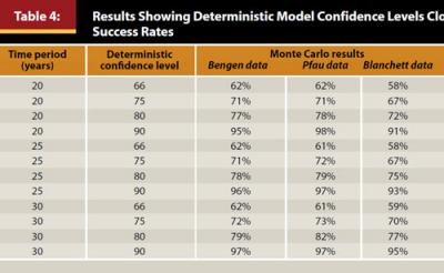
The deterministic model was tested to compare the results to Monte Carlo simulation with both methods using the same capital market inputs. Three different capital market inputs were obtained from the three research papers previously described (Bengen 1994; Pfau 2012; Blanchett et al. 2013).
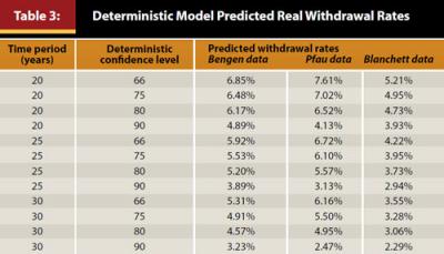
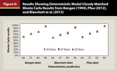
To test the model, first the deterministic model was used to calculate withdrawal payout rates using the derived geometric average return at all four levels of confidence (66, 75, 80, 90 percentiles) across 20-, 25-, and 30-year horizons. Thus, 12 withdrawal payout rates were calculated for each of the three studies’ capital market data. Next, 10,000 Monte Carlo success simulations were run using each of the 12 withdrawal payout rates to measure success probabilities. The deterministic model-predicted success rates (confidence level) were compared to Monte Carlo success results for each capital market dataset. The predicted deterministic model confidence level results were very closely aligned to the Monte Carlo success results, as shown in Tables 3 and 4 and Figure 6.
Using Derived Geometric Returns to Periodically Recalculate Withdrawal Rates
The deterministic method is especially useful for periodic resampling when using an adaptive approach to distribution planning. In such a process, the ongoing withdrawal rate is variable over time and not a constant, and as such, periodic reexamination of sustainable withdrawal rates can further improve the probability of success of a distribution strategy (Blanchett and Frank 2009). This adaptive approach concedes that sustainability decisions do not occur just once at retirement, but will almost certainly change as situations come up throughout retirement.
The deterministic model can be used to break down the full distribution period into several smaller sub units, such as five-year increments. The advantage is that when using the same inputs, unlike Monte Carlo, each repetitive deterministic calculation provides the exact same answer. Thus, any variability in the success answer or sustainable withdrawal rate can be attributed to the client’s changing situation, rather than the inherent randomness of the Monte Carlo process.
Impact of Fat Tails in the Deterministic Model
The deterministic model is based upon modern portfolio theory risk metrics, meaning that standard deviation is the definition of risk. For this concept to work best it requires a normal bell shaped curve of symmetrical distributions around the arithmetic average. Unfortunately, financial investment returns are a non-normal type of distribution curve and do not exactly fit to a bell curve (Swisher and Kasten 2005). The shape of the curve is not symmetrical, which gives rise to the term “fat tail.” This means that upside deviations are not the same as downside deviations.
The reason this is important is that a distribution phase fund that takes a 20 to 40 percent loss early in the payout phase will likely never recover and be sustainable. This is what many investors experienced in 2008. However, because these downside deviations are infrequent and generally outside of even the 90 percentile level of confidence, they do not materially affect the deterministic model any more than they affect Monte Carlo analysis. Fat tails can be mimicked by negatively adjusting the “z” values in combination with standard deviation to create greater downside deviations than would be predicted by normal distribution statistics. Financial planners wishing to further examine the impact of downside deviation risk (semivariance) and other non-normal distribution issues are encouraged to read Sortino and Satchell’s (2001) book on this subject.
Communication of Geometric Returns Withdrawal Rates
Explaining the retirement income management process involves much more than simply showing asset allocation or performance of a portfolio against a benchmark such as the S&P 500. Retirees are much more interested in the sustainability and reliability of their lifetime income stream.
Reporting should concisely communicate more to clients about how their retirement is progressing. The need to avoid jargon is important, and relative visual or graphical scales help communicate the message (Kasten and Kasten 2011). Client reports should be easy to understand with a graphical summary page and details placed in the body and appendix. The deterministic model is easily adapted to such customized reporting.
Conclusions
The deterministic model allows financial planners to easily incorporate customized withdrawal or success calculations into their proprietary workflows using a simple spreadsheet program. The method avoids the need to request custom and typically expensive programming in third-party financial planning software programs to meet a practice’s unique needs.
The simplified method uses portfolio standard deviation for conversion of arithmetic average return to the derived geometric average return for each level of confidence. Each confidence level has its own unique formulaic solution. The derived geometric equivalent return for a given level of desired confidence can be used to calculate the sustainable annual withdrawal. The deterministic model is stable, always reproducible, and highly correlated to Monte Carlo results. The deterministic method is especially useful for periodic resampling when using an adaptive approach to distribution planning, where the ongoing withdrawal rate is fluid and not constant. The approach can further improve the probability of success of a distribution strategy.
References
Athavale, Manoj, and Joseph M. Goebel. 2011. “A Safer Safe Withdrawal Rate Using Various Return Distributions.” Journal of Financial Planning 24 (7): 36–43.
Bengen, William P. 1994. “Determining Withdrawal Rates Using Historical Data.” Journal of Financial Planning 7 (10): 171–180.
Blanchett, David, Michael Finke, and Wade Pfau. 2013. “Low Bond Yields and Safe Portfolio Withdrawal Rates.” Morningstar.com.corporate.morningstar.com/us/documents/targetmaturity/LowBondYieldsWithdrawalRates.pdf.
Blanchett, David, and Larry R. Frank. 2009. “A Dynamic and Adaptive Approach to Distribution Planning and Monitoring.” Journal of Financial Planning 22 (4): 52–66.
Brayman, Shawn. 2007. “Beyond Monte Carlo Analysis: An Algorithmic Replacement for a Misunderstood Practice.” Journal of Financial Planning 20 (12): 56–73.
Kasten, Gregory W., and Michael W. Kasten. 2011. “The Impact of Aging on Retirement Income Decision Making.” Journal of Financial Planning 24 (6): 60–69.
Milevsky, Moshe A., and Anna Abaimova. 2006. “Will the True Monte Carlo Number Please Stand Up?” Journal of Financial Planning: Between the Issues. www.FPAnet.org/Journal/BetweentheIssues/LastMonth/Articles/WillTheTrueMonteCarloNumberPleaseStandUp/.
Nawrocki, David. 2001. “The Problems with Monte Carlo Simulation.” Journal of Financial Planning 14 (11): 92–106.
Pfau, Wade. 2012. “Capital Market Expectations, Asset Allocation, and Safe Withdrawal Rates” Journal of Financial Planning 26 (1): 36–43.
Sortino, Frank, and Stephen Satchell, eds. 2001. Managing Downside Risk in Financial Markets. Woburn, Massachusetts: Butterworth-Heinemann Publications.
Swisher, Pete, and Gregory W. Kasten. 2005. “Post Modern Portfolio Theory.” Journal of Financial Planning 18 (9): 74–85.
Turner, John A., and Hazel A. Witte. 2009. “Retirement Planning Software and Post-Retirement Risks.” The Society of Actuaries and The Actuarial Foundation. www.soa.org/research/research-projects/pension/retire-planning-software-post-retire-risk.aspx.
Citation
Kasten, Gregory W. 2013. “Using a Simplified Deterministic Model to Estimate Retirement Income Sustainability.” Journal of Financial Planning 27 (7): 56–62.