Journal of Financial Planning: August 2017
James S. Welch Jr. has been implementing mathematical programming systems since 1964. His interests are in matrix description languages, high-performance optimizers, and pre-solving models prior to optimization in order to speed the solution process. Since 1996, Welch has been acting as webmaster for the Optimal Retirement Planner website. He currently serves as a senior application developer for Dynaxys LLC.
Acknowledgements: The author thanks Beverly Barker, David S. Hirshfeld, William Burdick, and Eric Harding for their help with this manuscript; and Kanesha Hickman, Keisha Cato-Kanu, Cella Key, and Ashley Comer for their data-collection assistance.
Executive Summary
- Retirement planning involves coordinating income from multiple sources such that savings are not depleted prematurely, no large undesired surplus is left behind, and disposable income is maximized. This paper proposes a practical retirement savings withdrawal procedure using a free online calculator that addresses these objectives. The procedure is called 3-PEAT.
- The heart of 3-PEAT is a linear programming application that computes an optimal retirement income management plan whose results include annual savings withdrawals and maximum disposable income for the term of the plan.
- 3-PEAT requires that the retiree adapt to variable annual disposable income. The procedure increases withdrawals in rising markets and reduces withdrawals in down markets. Because it is a procedure, it is amenable to simulation.
- This paper analyzed 3-PEAT simulations for six historical stock market periods. Results show that when 3-PEAT was compared to other variable withdrawal methods, it increased disposable income, prevented savings from being depleted prematurely, and reduced the variability of annual disposable income.
Increasingly, due to the switch from employer-managed pensions to retiree-managed, tax-advantaged savings, more retirees have to coordinate income from multiple sources such that savings are not depleted prematurely, no large undesired surplus is left behind, and disposable income is maximized.
Some retirement plan participants have used various online retirement calculators to self-manage their retirement savings withdrawals. Users enter their parameters and compute a retirement plan that likely includes the optimal savings withdrawal for the current year. This paper proposes a practical retirement savings withdrawal procedure that formalizes what users of online calculators are doing on an ad hoc basis. The three-step procedure, called 3-PEAT1, uses linear programming (a rigorous optimization method) to compute the optimal annual savings withdrawal. The optimal plan maximizes disposable income by scheduling savings withdrawals in a manner that balances the minimization of taxes against the maximization of asset returns.
Following the literature review, the methodology is explained, 3-PEAT and the variable withdrawal simulator (VWS) are defined, and computational results are reported. The appendix demonstrates how VWS simulates a retiree using 3-PEAT to manage her retirement income for a 30-year retirement.
Literature Review
Retirees want both the stability of constant spending and the rewards of investing in equity markets (Finke and Blanchett 2016). Bengen (1994) was the first to address this issue with his now well-known 4 percent rule. He reported that fixing the annual withdrawal amount at 4 percent of initial savings, indexed to inflation, would fund a 30-year retirement. Current researchers seek methods that establish higher percentages of retirement savings that can be spent without increasing the probability of plan failure.
Guyton and Klinger (2006) introduced limited withdrawal variability into their inflation-indexed, constant-spending model. They began retirement with a heuristically determined initial withdrawal rate of some small percentage (e.g., 4 percent) of the initial retirement savings balance. From this they computed the initial withdrawal amount. Each year’s withdrawal amount was the initial withdrawal amount indexed to compounded inflation. They defined the year’s withdrawal rate to be the year’s withdrawal amount divided by the year’s savings balance. They then applied a set of decision rules to enhance the withdrawal rate so that plan failure was avoided. Their decision rules were based on the relative values of the initial withdrawal rate and the year’s withdrawal rate along with market returns and changes to the consumer price index. For some years this adjusted the year’s withdrawal rate which, in turn, adjusted the year’s withdrawal amount.
The difficulty with constant withdrawal rate methods, as noted by Guyton and Klinger (2006), is that throughout retirement, withdrawal amounts are tied to the initial withdrawal rate/amount that may have been unsuitable for a “perfect storm” economic environment that developed shortly after the initial withdrawal. This is the sequence of returns risk (Kitces 2014) when a reasonably constructed initial withdrawal amount turns out to be inappropriate for a difficult economic environment that occurs after retirement begins.
Guyton and Klinger (2006) observed that plan failures tended to occur more often later in retirement and were caused by overly generous withdrawals early in the plan. They also identified a little-recognized hazard in plans that did not fail but suffered from reduced purchasing power late in retirement due to an adverse inflationary environment.
Other researchers abandoned the constant spending constraint and allowed for variable spending tied to changes in savings valuation; the stock market goes up—spend more, the market goes down—spend less (Pfau 2015b).
Delorme (2015) offered a “blueprint” for assigning a retirement income management method to a retiree’s preference. His blueprint combined two withdrawal methods (constant and flexible) with two client risk preferences (safe and optimal). Delorme’s safe option protected against plan failure by sacrificing spending in favor of a final total asset balance surplus. His optimal option increased disposable income by allowing for variable spending. Delorme offered three computational methods:
Constant was basically Bengen’s 4 percent rule with the initial constant withdrawal amount set to 3.8 percent of the beginning savings balance. This withdrawal amount was set at the beginning of the plan and, with inflation adjustments, retained regardless of anything that happened thereafter.
Flexible – RMD+ was an augmented IRS required minimum distribution calculation where the annual withdrawal was the savings balance divided by an age-related constant from a table supplied by the IRS, plus 2.7 percent.
Flexible – Fixed Percentage (FP) withdrew 5.6 percent of remaining savings every year of retirement, adjusted for inflation.
Delorme (2015) found that the flexible methods adapted to changing savings balances; they did not suffer from plan failures.
Methodology
The procedure proposed in this paper will not fully deplete saving prematurely, nor will it end with an unwanted surplus because it treats each plan’s final total asset balance as a constraint. The procedure, 3-PEAT, varies annual disposable income according to the value of retirement savings, plan length, and inflation. It confines retiree spending to within the limits of varying levels of disposable income, thereby avoiding prematurely depleting retirement savings.
Because 3-PEAT is a procedure, it is amenable to simulation. The variable withdrawal simulator (VWS) simulates the actions of a retiree using 3-PEAT to execute a 30-year retirement plan. This paper analyzed the results of experiments performed using VWS. Download the VWS spreadsheets for this study at www.i-orp.com/3-peat/3-peat.xlsx.
Bengen’s (1994) idea of back-testing over historic stock market periods was adopted using Shiller’s S&P 500 index database (available at www.econ.yale.edu/~shiller/data.htm). VWS’s essence is to operate 3-PEAT as though the present-day retirement framework of tax-advantaged accounts, Social Security income indexed to inflation, progressive taxation, index funds, etc., existed in historic market situations where most of these features had yet to be implemented. Six historic periods were chosen for this study:
Modern Era (1985 to 2015) included the dot.com bubble and the Great Recession.
Bengen’s Big Bang (1973 to 2003) began with the 1973 sell-off. Guyton and Klinger (2006) named this period the “perfect storm” because “… it included a severe market decline in the initial retirement years combined with inflation in the first decade of retirement that was three times the long-term historical norm” (page 49).
Stagflation (1966 to 1996) was a period of mediocre market performance, high inflation (by U.S. standards), and a stagnant economy.
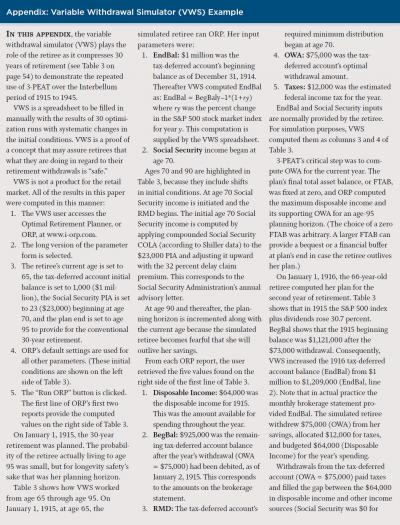
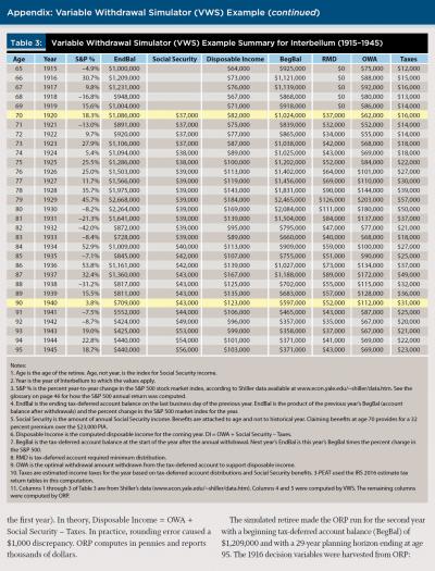
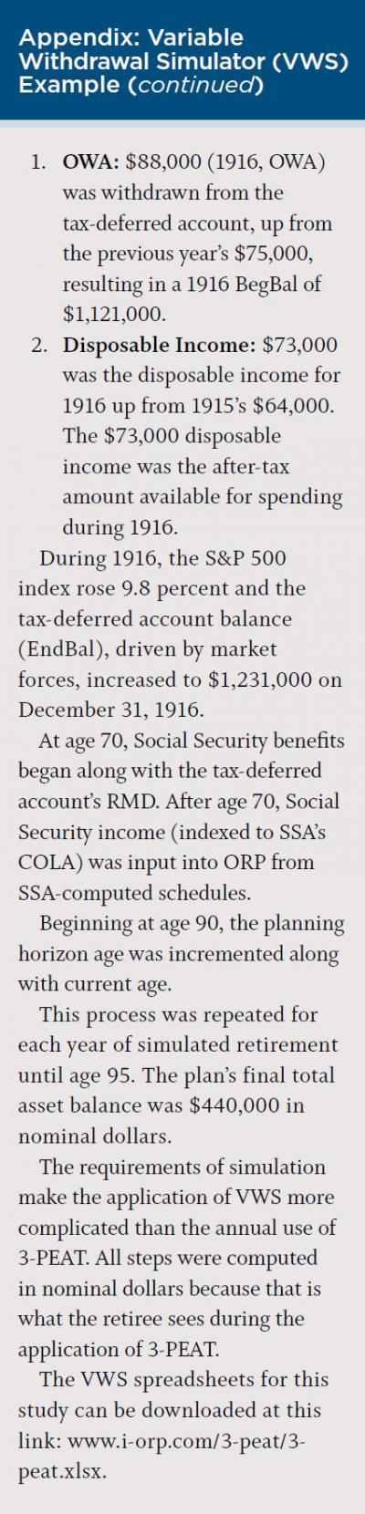
Interbellum (1915 to 1945) as defined for the purpose of this paper, was the period where two World Wars bookended the Great Depression.2
Worst-Case (1903 to 1933) was one of only two 30-year retirement periods in which the S&P 500 index finished lower (7.09) than it began (8.46) for a slope of –0.05. The other, which began three years before Interbellum, had a slope of –0.01.
Gilded Age (1880 to 1910) featured the panics of 1901 and 1907 (Richardson and Sablik 2015).
The annual retirement plans computed for each era were optimal, i.e. there was no mathematically superior solution to the annual plans (Dantzig 1963). The 30-year plan was feasible in that it did not fail, it did not leave a large, unplanned surplus at the end, and it minimized the amount of downside variability in its computed disposable incomes.
Linear Programming Applications
Before describing how 3-PEAT works, it is important to understand the nature of the underlying mathematical programming. At the core of the 3-PEAT procedure is the Optimal Retirement Planner (ORP), a free, online retirement calculator available at www.i-orp.com.
ORP is a linear programming (LP) application that finds the optimal solution for conflicting requirements. Linear programming is a mathematical tool where a process is modeled as a set of linear equations. Normally there are more variables than equations; this means there are many solutions to the equations. The objective function is the linear function that spans the entire system and assigns a cost or profit to each variable in the system. This function computes the profit for a solution to the system of equations. The optimal solution is one with the maximum value of the objective function.
The genius of linear programming is the simplex method (Dantzig 1963) that evaluates a relatively small number of candidate solutions as it seeks the optimal solution, which is guaranteed to maximize the objective function.
Ragsdale, Seila, and Little (1994) and Coopersmith and Sumutka (2011) demonstrated that the linear model is a suitable representation of the retirement income management process. They each laid out the retirement model in algebraic form. The competing forces of the retirement income model are minimizing taxes (cost reduction) and maximizing compounded asset returns (profit maximization). Linear programming finds the optimal balance between these two objectives. The pivotal constraint is the constant disposable income, indexed to inflation, assumption.
ORP’s problem definition is opposite that of conventional practice. Other retirement calculators reported in the literature fixed spending at some a priori value and computed the final total asset balance, or FTAB. They used FTAB to measure the efficiency of competing plans; the larger the FTAB, the better the plan. ORP fixes the FTAB and maximizes disposable income based on the user-supplied initial conditions.
Welch (2015a) validated the linear programming approach that fixed FTAB and maximized disposable income. That analysis demonstrated linear programming’s advantage over the conventional savings withdrawal practice of distributing the taxable account until depletion, then the tax-deferred account, followed by the Roth IRA.
Computer programming developer Wayne Scott constructed a linear programming-based retirement calculator using the Python programming language that focuses on early retirement issues such as the 10 percent early withdrawal penalty, the 72(t) exception to the early withdrawal penalty, and the timing of Roth IRA withdrawals. Although the experiments reported in this paper were done using ORP, Scott’s calculator (free and readily available at github.com/wscott/fplan) could have served just as well.
Linear programming, or LP, retirement optimizers are a generation beyond many of the simulators currently in use (for example, the IRS 1040 tax table is integrated into LP optimizers, so tax-efficient results are more relevant to retirement income planning), and they offer a “sandbox” for experimentation with various savings withdrawal strategies.3
Modest LP formulation skills are required to implement an LP retirement model. Several commercial or open source LP model generators and solvers are available to support such development.4 Research into retirement income management should consider exploration in this direction.
How 3-PEAT Works
3-PEAT shares basic principles with other variable withdrawal methods. They all compute the withdrawal amount based on remaining assets and time to the end of the planning horizon. The fundamental difference is that 3-PEAT replaces the arithmetic withdrawal functions with a comprehensive optimization that takes more factors, such as progressive income taxes or delaying Social Security income to age 70, into consideration when computing each year’s withdrawal.
3-PEAT is a manual procedure for managing retirement income. 3-PEAT’s three steps are:
Step 1: The retiree determines her current savings account balance from her monthly brokerage statement, her Social Security benefits from SSA’s annual benefits advisory letter, and her age from her birth certificate.
Step 2: She logs onto www.i-orp.com and runs the Optimal Retirement Planner, or ORP, (the readily available linear programming application that computes her full retirement plan) using the input parameters from Step 1 along with other information that provides personal details of her retirement situation.
Step 3: ORP reports an income management plan for the specified retirement duration. The report shows annual disposable income and specifies withdrawals for every year of the plan. The retiree withdraws the amount reported as the plan’s first-year distribution from her savings and budgets her annual spending to fit the plan’s first-year disposable income.
Next year, when the retiree is a year older, she repeats the process, again taking the actions indicated for the first year of her new retirement plan. The step 3 reports are just guidelines for income management. Final cash management decisions should be based on personal preferences and legal factors beyond the scope of the model; ORP simply provides a sense of direction for the process.
The underlying logic of 3-PEAT is that ORP, using personal data specific to the retiree, projects a retirement income management plan to the planning horizon. The new plan maximizes disposable income, indexed to inflation, in a tax-efficient way across the remaining span of retirement. The retiree’s decision-making horizon is the current year. The retiree may be most comfortable making decisions for the current year only, because assumptions about the economic environment one year out can generally be made with more confidence than those five or 10 years out.
Following the adage: many people say they don’t want to live to be 95, but none of them are 94, the variable withdrawal simulator, or VWS, assumes that when the retiree turns age 90, she reconsiders her age-95 planning horizon and increases it to age 96. This is repeated every year until 3-PEAT’s plan ends at age 95. This leaves a modest savings balance at the end of the plan that is likely sufficient to support the retiree should she outlive the plan, but her final total asset balance is not depleted nor excessive. From a modeling perspective, this avoids a discontinuity at the end of the plan that distorts the final year’s results.
Computational Results
The following sections summarize 3-PEAT’s behavior under a variety of conditions. First is a presentation of results for the Interbellum period (1915 to 1945). Second is a comparison of 3-PEAT to Delorme’s (2015) three withdrawal methods, described earlier, for each of the chosen historic periods.
Assumptions. The retiree being modeled was assumed to be single, 65 years old, with $1 million in a tax-deferred account (TDA), and Social Security as her only other retirement asset. Her TDA was invested in an index fund that tracked the S&P 500.
A 100 percent equity index fund was chosen to bring out the effect of market volatility on savings withdrawals. 3-PEAT’s results for the all-equity portfolio serves as an upper limit for less-dynamic portfolios. “Savings” is used here to refer to the sum all retirement savings accounts including the TDA, Roth IRA, and taxable accounts.
The retiree’s Social Security income assumed that her principle insurance amount was $23,000. She claimed her benefits at age 70 and enjoyed the 32 percent delayed starting credit (Pfau 2015a).
3-PEAT’s disposable income was affected by two exogenous factors: (1) stock market returns; and (2) inflation. For stock market returns, changes in savings value—as measured by the change in the S&P 500 in this study—affected the size of the annual savings withdrawal. For inflation, Social Security’s cost of living adjustment (COLA) affected Social Security income.
3-PEAT Cash Flow
This section describes results for the Interbellum period as shown in the S&P 500 panel of Figure 1. (Additional results, including cash flow graphs for all eras, can be found at www.i-orp.com/3-PEAT/3-PEATsupplement.pdf). The slope of the line connecting the end points of Interbellum’s market index was a gentle 0.45, but the index was volatile over the 30 years. The average index return was 10.0 percent, and the annual return’s standard deviation was 23.4 percent. Bengen (1994) named two multi-year, severe market downturns in Interbellum. The “Little Dipper” began with the 1929 stock market crash, and he named the 1937 sell-off the “Big Dipper.”
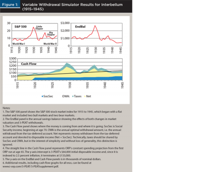
The EndBal panel of Figure 1 graphs the tax-deferred account’s annual ending balances across retirement. The low point, which occurred during the Little Dipper, was above $700,000, leaving sufficient savings for appreciation during the subsequent economic recovery. The account recovered before the Big Dipper began and, coincidently, the end-of-plan liquidation began. At the end of the plan (age 95) the tax-deferred account retained $437,000 to sustain disposable income to age 101, if needed. This proved to be a sufficient end-of-plan cushion, because between 1945 and 1952 the S&P 500 rose 57 percent.
The Cash Flow panel of Figure 1 shows 3-PEAT’s net was at a high level before age 70 when Social Security income began (net was the optimal withdrawal amount minus taxes). Social Security income cut the net and the optimal withdrawal amount in half. The early-period market was stable and net grew gradually until the roaring ’20s when growth accelerated. The 1929 crash contracted the net.
The initial ORP run at the beginning of retirement, with a 6 percent rate of return and 2.5 percent inflation, projected total disposable income over all of retirement (with zero FTAB) at $2,927,000, while 3-PEAT’s total disposable income plus FTAB was $3,736,000. Net’s low point at $46,000 was not during the Great Depression, but came later in 1943. Thanks to the Social Security COLA, DI’s low point did not come during the Depression.
The appendix on page 53 demonstrates how the variable withdrawal simulator was used to perform the calculations that resulted in Figure 1.
Comparing Withdrawal Methods
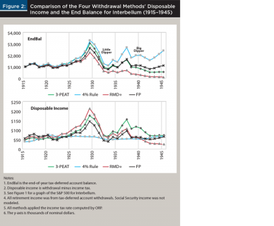
The following section compares 3-PEAT to three of Delorme’s (2015) savings withdrawal methods as described earlier. Disposable income and the end balance are shown for the four methods in Figure 2. Interbellum (1915 to 1945) was chosen as the time span for this comparison, because of its two traumatic market events. This discussion is an extension of the 3-PEAT results presented earlier in Figure 1.
Figure 2 gives the illusion that before the event dubbed the “Little Dipper,” all variable withdrawal methods were approximately the same. This is partially because the y-axis is scaled to the 1928 bubble, which obscures the volatility of the roaring ’20s.
Other key findings from this comparison include:
The 4 percent rule’s disposable income had low variability, fluctuating according to the CPI, but its end balance (EndBal) was as volatile as the others. Although the 4 percent rule under-withdrew and left a FTAB of $2.4 million, it did not fail during Interbellum.
Withdrawing too little left the fixed percentage (FP) method with a large FTAB of $757,000. Toward the end of the plan, FP’s large EndBals and a rising market increased this method’s disposable income.
The required minimum distribution is designed by the IRS to drive the tax-deferred account balance toward zero, so that the government can collect those deferred taxes. At mid-plan, the RMD+ method’s EndBal goes into descent as a result of its algorithm. By age 95, this withdrawal method’s EndBal is nearly zero. As the RMD+ method’s EndBal declined, so did its disposable income.
3-PEAT directed EndBal toward zero, thanks to ORP’s zero FTAB constraint. Near Interbellum’s end, 3-PEAT’s EndBal leveled off as the retiree extended her plan horizon each year after age 90. 3-PEAT did not have the highest disposable income before the Little Dipper but, because of its smaller withdrawals during that period, 3-PEAT’s disposable income exceeded the others during the Big Dipper.
Interbellum ended with a recovering stock market. The four methods responded to the recovery with four different performances.
The next section compares the wealth added to retirement income by the four withdrawal methods.
Measuring Plan Worth
The economic worth of a withdrawal method can be measured by its total disposable income over the duration of the plan. Table 1 compares the disposable income for the four methods across the six time periods defined in the methodology section.
The 4 percent rule suffered two plan failures (indicated by blank entries in Table 1). The fixed percentage (FP) and 3-PEAT methods are immune to plan failure. Table 1 shows that the plans’ results are sensitive to the method used to compute withdrawals. The 4 percent rule’s total withdrawals during the Modern Era suffered from a combination of a strong stock market, which it ignored, and low inflation, which held down its annual disposable income increases.
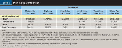
The Stagflation period was a difficult period to be retired. The initial savings balance in 1973 was $1 million, but only $985,000 (real) was available for disposable income; the remainder went to pay taxes. All other periods distributed substantially more than the initial balance as disposable income. Recall that there was no Social Security income for these tests and that the values in Table 1 are real—the effects of inflation have been removed.
Measuring Plan Variability
A plan’s psychological worth—that is, making the retiree comfortable with withdrawing from her retirement savings—can be measured by how much disposable income variability she has to endure. The retiree’s expectation is that her initial disposable income is indicative of her annual disposable income throughout retirement. It may become a source of concern when her withdrawal method reduces a year’s disposable income below her initial disposable income.
Table 2 offers two measures of method variability. Panel A of Table 2 is the retiree’s discomfort index—the more negative the Panel A percentage, the higher the discomfort. The larger the Panel B count, the longer the discomfort lasts.
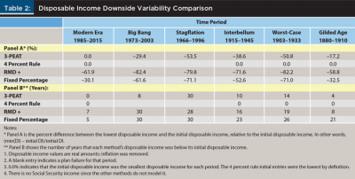
Some researchers, including Kitces (2012), separate retirement spending into essential and discretionary spending. Essential spending is commonly expenses that have to be met, such as food, shelter, and clothing. Discretionary spending is commonly optional spending that can be foregone, such as cruises or golf.
The message of Panel A in Table 2 is that if essential spending exceeds 50 percent of disposable income, then the prospective retiree is not financially ready for retirement. In summary, Table 2 shows that 3-PEAT produced the highest total disposable income and lowest total disposable downside variability.
Using 3-PEAT in Real Life
At the beginning of each year, 3-PEAT reports the optimal withdrawal amount as a single value. The married retiree decides whether to withdraw from her tax-deferred account, her spouse’s account, or both; the choice does not matter to 3-PEAT. The only requirement is that their two separate RMDs are met.
The 3-PEAT user enjoys a certain amount of latitude in deviating from 3-PEAT’s plan:
- Withdrawals from the wrong account may divert the plan from the optimal path but is otherwise not fatal.
- Withdrawing more than 3-PEAT’s recommended amount for essential spending is effectively stealing from the future. If done with discretion, this would reduce total disposable income, but if done in excess, it would deplete the end balance, which is plan failure.
- Withdrawing less than the recommended amount leaves larger account balances for the lean years. If the withdrawals are less than the RMD, then the difference is transferred to the taxable account.5
The retiree’s withdrawals would be reflected in the initial account balances for the forthcoming year (3-PEAT’s Step 1). Tax-deferred account withdrawals are assumed to take place at the first of the year. In fact, they can take place anytime during the year with little effect on the plan’s overall outcome.
Conclusion
3-PEAT has been shown here to be a practical, safe procedure for managing income over the term of retirement. The procedure avoids plan failures caused by premature savings depletion. Compared to other variable withdrawal methods analyzed in this paper, 3-PEAT increased disposable income and reduced income variability. Its computed disposable income varied from year to year because of variable savings withdrawals, changes in asset market valuation, and inflation-induced changes in Social Security benefits.
3-PEAT immunized a retirement savings plan from plan failure and increased the total amount of disposable income relative to the other withdrawal methods tested. Although 3-PEAT increased disposable income over the planning period, it did not necessarily maximize it. There may be even better plans with larger total disposable income.
Retirees face a psychological challenge as they enter retirement. They may have considerable angst when retirement savings stop growing and begin to be consumed. 3-PEAT may be an important tool to help financial advisers help clients adjust to consuming savings. This paper has shown that 3-PEAT is a withdrawal method that will not prematurely deplete retirement savings and will reduce year-to-year disposable income variability.
The do-it-yourselfers known to the author to be practicing their own form of 3-PEAT are engineers and accountants, a population that in many cases already has some acquaintance with linear programming and is comfortable with quantitative methods. This leaves a rather large population of retirees who financial advisers may comfort with the assurance that 3-PEAT is mathematically sound and has been shown to not have deserted them during known difficult market conditions. The fearful may be assured that the math is on their side.
Endnotes
- 3-PEAT is not a commercial product nor a procedure used for commercial purposes; it should not be confused with the trademarked 3-Peat for clothing and sports memorabilia.
- Interbellum is commonly defined as the period between the end of World War I (1918) and the beginning of World War II (1939). In order to get a 30-year retirement span, the two World Wars were included in Interbellum in this analysis.
- Examples of linear programming-based retirement calculators include the Optimal Retirement Planner, available at www.i-orp.com; and the Early Retirement Financial Calculator, available at github.com/wscott/fplan. Research that has used linear programming methods include: Ragsdale, Seila, and Little (1994); Coopersmith and Sumutka (2011); (Welch 2015b); Welch (2016); and Coopersmith and Sumutka (2017).
- FICO’s XPRESS/MP (fico.com) provides a martrix description language and top-of-the-line solver. GLPK (gnu.org/software/glpk) is a GNU open source matrix description language, and lp_solve (lpsolve.sourceforge.net/5.1) is a GNU open source solver.
- Floor-and-ceiling withdrawal tactics violate 3-PEAT’s program in the interest of smoothing savings withdrawals and meeting essential spending requirements. This is discussed more fully in a working paper available at i-orp.com/3-PEAT/FandC.pdf.
References
Bengen, William P. 1994. “Determining Withdrawal Rates Using Historical Data.” Journal of Financial Planning 17 (3): 172–180.
Coopersmith, Lewis W., and Alan R. Sumutka. 2011. “Tax-Efficient Retirement Withdrawal Planning Using a Linear Programming Model.” Journal of Financial Planning 24 (9): 50–59.
Coopersmith, Lewis W., and Alan R. Sumutka. 2017. “The Impact of Rates of Return on Roth Conversion Decisions and Retiree Savings Wealth.” Journal of Personal Finance 16 (1): 29–39.
Dantzig, George B. 1963. Linear Programming and Extensions. Princeton, N.J.: Princeton University Press.
Delorme, Luke. 2015. “A Blueprint for Retirement Spending.” Journal of Financial Planning 28 (9): 40–50.
Finke, Michael, and David Blanchett. 2016. “An Overview of Retirement Income Strategies.” Journal of Investment Consulting 17 (1) 22–30.
Guyton, Jonathan T., and William J. Klinger. 2006 “Decision Rules and Maximum Initial Withdrawal Rates.” Journal of Financial Planning 19 (3): 48–58.
Kitces, Michael. 2012. “The Problem with Essential-Vs-Discretionary Retirement Strategies.” Nerd’s Eye View, posted May 30 at kitces.com/blog/the-problem-with-essential-vs-discretionary-retirement-strategies.
Kitces, Michael. 2014. “Understanding Sequence of Return Risk—Safe Withdrawal Rates, Bear Market Crashes, and Bad Decades.” Nerd’s Eye View, posted October 1 at kitces.com/blog/understanding-sequence-of-return-risk-safe-withdrawal-rates-bear-market-crashes-and-bad-decades.
Pfau, Wade D. 2015a. “The Case for Delaying Social Security.” Journal of Financial Planning 28 (10): 42–51.
Pfau, Wade D. 2015b. “Making Sense Out of Variable Spending Strategies for Retirees.” Journal of Financial Planning 28 (12): 28–30.
Ragsdale, Cliff T., Andrew F. Seila, and Philip L. Little. 1994. “An Optimization Model for Scheduling Withdrawals from Tax-Deferred Retirement Accounts.” Financial Services Review 3 (2): 93–108.
Richardson, Gary, and Tim Sablik. 2015. “Banking Panics of the Gilded Age.” Federal Reserve History. Available at federalreservehistory.org/Events/DetailView/98.
Welch, James S. 2015a. “Mitigating the Impact of Personal Income Taxes on Retirement Savings Distributions.” Journal of Personal Finance 14 (1): 17–27.
Welch, James S. 2015b. “A Quantitative Evaluation of Four Retirement Spending Models.” Journal of Personal Finance 14 (2): 43–57.
Welch, James S. 2016. “Measuring the Financial Consequences of IRA to Roth IRA Conversions.” Journal of Personal Finance 15 (1): 47–55.
Citation
Welch, James S. Jr. 2017. “A 3-Step Procedure for Computing Sustainable Retirement Savings Withdrawals.” Journal of Financial Planning 30 (8): 45–55.