The Social Security Claiming Decision for Married Couples

Journal of Financial Planning: December 2025

Executive Summary

• Married couples optimizing the Social Security claiming decision must account for possibly two worker benefits, a spousal benefit, and a potential survivor or widow benefit. The set of monthly claim age combinations available to them can exceed 9,000, not including options for claiming survivor benefits. This is a far more complex consideration than for individuals who need only select a single claim age.
• Optimal claiming strategies are examined here for married couples spanning a wide range of age differences, covering the entire spectrum of relative lifetime earnings between the spouses, and for all valid monthly claim age combinations in each case.
• Results indicate that for couples with the traditional situation of an older, higher-earning husband, optimal claim strategies always consist of a delay by the husband, usually to age 70, and an early claim by the wife, almost always at age 62. If the higher-earning husband is younger, however, optimal claim strategies are highly variable over the range of spousal age gaps and earnings ratios, often suggesting the reverse with the husband claiming early and the wife delaying. This result is particularly true for couples with near equal earnings.
• As the future lifetime earnings gap between husbands and wives continues to narrow, the findings of this study for couples with near equal lifetime earnings should be of increasing interest and importance.

Brian J. Alleva is a research analyst at the Social Security Administration. He specializes in retirement income and related policy analysis, primarily using stochastic modeling and simulation, machine learning, and data science techniques. He recently produced a publicly available synthetic microdata set of benefits and earnings figures for the Social Security beneficiary population.

Disclaimer: The findings and conclusions presented in this manuscript are those of the author and do not necessarily represent the views of the Social Security Administration or any federal agency.

NOTE: Click on the images below for PDF versions.

JOIN THE DISCUSSION: Discuss this article with fellow FPA Members through FPA's Knowledge Circles​​​​. ​​​

FEEDBACK: If you have any questions or comments on this article, please contact the editor HERE. 

Never-married workers eligible for Social Security retirement benefits can choose between 97 monthly claim ages from 62 to 70, with the lifelong monthly benefit amount amount increasing for each successive claim age. In contrast, the claiming considerations for married couples present a level of complexity far exceeding that for an individual. Depending on the birth years and earnings histories of the two spouses, the set of valid claim age combinations available to them can exceed 9,000, not including options for claiming survivor benefits (Alleva 2017).

One way to determine an optimal claim strategy is to maximize the expected present value of lifetime benefits.¹ For married couples, this method requires (1) an account of the age difference between the spouses and their respective survival expectations, (2) their earnings ratio, or the ratio of the lifetime earnings of the lower earner in the couple to that of the higher earner, and (3) a discount rate with which to value the benefit cash flows. Several previous studies of claiming strategies for married couples used this methodology (Shoven and Slavov 2014a, Shoven and Slavov 2014b, Sass et al. 2007, Munnell and Soto 2007, Meyer and Reichenstein 2010).

The general conclusion of these studies is that the higher earner in the couple, traditionally an older husband, should delay claiming his own worker benefit, often until age 70, and the lower earner, traditionally a younger wife, should claim her own worker benefit early if not immediately at 62. Delay of the older, higher-earning husband’s worker benefit increases the future widow benefit, effectively buying the couple a second-to-die or joint life annuity, which can weigh heavily in the couple’s total expected lifetime benefits. The wife’s worker benefit stream, which would be replaced by her husband’s worker benefit at his death, is essentially a first-to-die annuity. As such, it is usually maximized with an early claim because the husband is expected to die well before his wife and recouping from any delay of her worker benefit is unlikely.

Munnell and Soto (2007), Meyer and Reichenstein (2010), Shoven and Slavov (2014a), and Sun and Webb (2011) found this claiming strategy especially favorable for couples with a much younger wife, whose life expectancy is much longer at retirement than that of her husband, but less so when they are closer in age and the expected period of widowhood is much shorter. Munnell and Soto (2007) also found that the higher the couple’s earnings ratio, the longer the husband should delay. The wife, however, should only delay beyond 62 at lower earnings ratios, and then only if close in age to the husband. The results of Sun and Webb (2011) differed somewhat but led to the same general conclusion that the gap between the optimal claim ages of the husband and wife widens as the earnings ratio increases.

The present study extends previous research in several ways. First, optimal claiming strategies are examined for a wider range of age differences between the husband and wife, including cases where the husband is younger, which have not been explored much previously.

Secondly, optimal claiming strategies over the full spectrum of earnings ratios, from single earner to equal-earner couples, are explored in depth for each sample couple. Iams (2016) found that the average gap between the lifetime earnings of husbands and wives has been closing in recent generations. Over 80 percent of married women entering retirement are now expected to have earned enough to rely solely on their own worker benefit while married in retirement, and about 30 percent to retain that worker benefit into widowhood as it will exceed the otherwise available widow benefit. Thus, a closer examination of couples with similar lifetime earnings between husband and wife should be of increasing interest.

Overall, results here are generally consistent with prior studies but with some surprising exceptions. For couples with the traditional situation of an older, higher-earning husband, optimal claim strategies always consist of a delay by the husband, usually to age 70, and an early claim by the wife, almost always at age 62. However, if the higher-earning husband is younger, the results can be highly variable over the spectrum of earnings ratios, often with sharp inversions of the optimal claim ages. Above a certain earnings ratio, dependent on the couple, the husband’s optimal claim age is 62 while the wife’s optimal claim age is 70. This finding suggests that, as the future lifetime earnings gap between husbands and wives continues to narrow, the usual advice of a high-earner delay and a low-earner immediate claim should be made with some reservation.

Thirdly, whereas previous studies examine claim strategies that optimize over the full retirement horizon through death of the widow, this study also breaks the full period into its constituent joint period when both spouses are alive, and survivor period when only one spouse is alive, for further analysis. As might be expected, optimal claim ages for the joint period, with very few exceptions, are the same or younger than those for the corresponding full retirement period. Conversely, survivor period optimal claim ages are invariably the same or older than those for the full period.

Methods

This study considers a series of married couples of varying age differences. Each couple consists of the traditional structure of a higher-earning male husband married to a lower-earning female wife. Social Security rules apply to all participants equally without regard to sex. The only differences between the sexes in this study are the survival functions. Tests using the wife as the high earner instead of the husband showed similar results and trends over the age differences and earnings ratios, indicating that the difference in survival functions between the sexes plays a minor role in determining the optimal claim strategy.

In each couple, the older spouse, either the husband or the wife, is aged 62 years in 2024 and so was born in 1962. The series accounts for a range of annual age differences between the husband and wife from +10 (husband is older) to −10 (wife is older), including the same-age couple in which both are born in 1962. A given couple is indicated with the notation [husband birth year, wife birth year], or alternatively [husband age in 2024, wife age in 2024]. The full series of couples with relevant information is listed in Table 1.

With the above specification, neither spouse in 2024 is older than 62, the earliest age to claim worker benefits, so all couples can consider the full set of claim age options available to them for optimization. Year 2024 is the reference year, or the year the couple is assumed to make the decision of when to claim their respective benefits and the year to which all present values are calculated.

Survival Functions

Each couple’s joint survival function is required for computing the expected present value of lifetime benefits. Though the younger spouse in each couple will reach age 62 sometime after reference year 2024 (except for the couple with spouses of the same age), all spouses in this study are assumed to survive to at least age 62 and die by age 120. Thus, for a spouse of a given sex born in a given year, his or her survival function consists of the probability of surviving to each annual age from 62 to 120 upon having attained age 62. Based on these survival functions,² Table 1 lists, for each spouse of each couple, the expected number of years of life remaining (life expectancy) as of the reference year, assuming survival to at least age 62.

 Joint survival functions for each couple are based on the probabilities of their possible death outcomes, or the set of all possible pairs of death ages between the spouses. Since each spouse in this study can die at any age between 62 and 120, there are [(120−62)²]  or 3,364 annual aged death outcomes for each couple. As a necessary simplification for this study, the death probabilities of the spouses are assumed to be independent and exclude consideration of any effects of marriage on spousal survival. Accordingly, the probability of each death outcome itself is the probability of the husband’s death age of the outcome multiplied by the probability of the wife’s death age of the outcome. Though each couple has the same set of 3,364 death age outcomes, the probability of each outcome varies by couple as the survival function of each spouse is dependent on both birth year and sex. The probability that a given spouse in a couple will be the survivor can be determined directly from the relevant death outcome probabilities. Table 1 lists, for each couple, the probability of each spouse as the survivor.

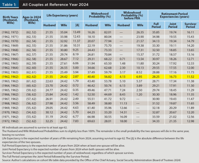
For a given death outcome, the full period of retirement is from the reference year until the death of the surviving spouse and specifies the number of years at least one spouse is alive. This full period comprises the joint period followed by the survivor period. The joint period is from the reference year until the first death and specifies the exact number of years both spouses are alive together. The survivor period is from the first death until the death of the surviving spouse and specifies the number of years when exactly one spouse is alive. Note that if both spouses die simultaneously (or in the same year, as all death ages are annual in this study), there is no survivor period and the full period consists solely of the joint period. If either spouse dies during the reference year (that is, they attained age 62 but died before age 63), there is no joint period, only a survivor period. With the full, joint, and survivor periods of each possible death outcome determined for a given couple, the period expectancies, or expected durations, of the couple’s full, joint, and survivor periods are computed from the death outcome probabilities and are shown in Table 1 for each couple.³

Worker and Spousal Benefit Claiming Rules and Formulas

The primary insurance amount (PIA) is the monthly benefit amount for an eligible worker who claims at their full retirement age (FRA).⁴ The PIA is determined from the worker’s aggregate lifetime earnings. The FRA is defined by birth year irrespective of sex. For cohorts born in 1960 and later, the FRA is age 67. Thus, for each birth cohort referenced in this study, the FRA is 67.

Each spouse eligible for a worker benefit can claim that benefit at any monthly age between 62 and 70 independently of the worker benefit claiming choice of the other spouse. If the worker benefit is claimed at the FRA, the monthly benefit amount is the PIA. If a worker benefit is claimed before the FRA, the monthly benefit amount is the PIA reduced by 5/9 of one percent for each of the first 36 months before the FRA, and 5/12 of one percent for each additional month down to age 62. If the benefit is claimed after the FRA, the monthly benefit amount is the PIA increased by 2/3 of one percent for each month beyond the FRA up to age 70.

For this study, all workers are assumed to have ceased covered work as of age 62, keeping both the PIA (calculated as of age 62) and the monthly benefit amount constant throughout retirement. There are numerous complicating factors affecting the benefit calculation and timing of receipts if covered work were to continue after claiming. These include the possibilities of benefit taxation, “earnings test” withholding, and periodic PIA re-computation, all of which could substantially affect benefit cash flows after claiming and thus determination of the optimal claim strategy. It should be noted also that the PIA and benefit amount remain fixed throughout retirement only in real terms through an annual cost-of-living adjustment, which is accounted for here by expressing all benefit cash flows and discount rates (see below) in real terms.⁵

The high earner in a couple is the spouse with the higher lifetime earnings and thus the higher PIA. Likewise, the low earner is the spouse with the lower PIA. For optimization considerations, only the relative value of the two PIAs, the PIA ratio, is relevant, and is expressed as the PIA of the low earner as a percentage of the PIA of the high earner. If the low earner has insufficient lifetime earnings to qualify for a PIA of her own, the PIA ratio is zero. If both spouses have equal lifetime earnings and thus equal PIAs, the PIA ratio is 100.

If the PIA ratio is less than 50, the low earner is eligible for an additional spousal benefit calculated to bring her total benefit to half that of the high earner, assuming all claiming is at the respective FRAs. As such, the spousal PIA here refers to the spousal benefit as a percentage of the high earner’s PIA. If the PIA ratio is zero, the spousal PIA is 50 and the low earner (and couple) is defined as spousal-only. If the PIA ratio is greater than zero but less than 50, the spousal PIA is 50 minus the PIA ratio, and the low earner is dually entitled as she is eligible for both a worker benefit of her own and a spousal benefit. If the PIA ratio is 50 or greater, she is not eligible for a spousal benefit, so the spousal PIA is zero and the low earner is worker-only.

If the spousal benefit is claimed at the FRA, the monthly spousal benefit amount is the spousal PIA. If the spousal benefit is claimed before the FRA, the spousal benefit amount is the spousal PIA reduced by 25/36 of one percent for each of the first 36 months before the FRA, and 5/12 of one percent for each additional month down to age 62. Unlike the worker benefit however, if the spousal benefit is claimed after the FRA, there is no increase, and the spousal benefit amount is the spousal PIA itself.

The age the high earner claims his own worker benefit (HCA), the age the low earner claims her own worker benefit (LCA), and the age the low earner claims the spousal benefit (SCA) are expressed here in the format years:months of age, or simply years of age if the claim age were to occur on an annual birthday. A dually entitled low earner must claim any spousal benefit at the later of her LCA and the calendar month of the HCA. This means that the spousal benefit may only be claimed when or after the high earner claims his worker benefit, even if the low earner is required to delay the SCA beyond her FRA to no advantage. In the event the HCA occurs later than the LCA, the spousal benefit claim is HCA-restricted. A spousal-only low earner can claim the spousal benefit, provided she has reached age 62, at or at any time after the HCA.⁶

Widow Benefit Claiming Rules and Formulas

The widow benefit formula is far more complex than either the worker or the spousal benefit formula. The widow benefit amount is dependent on both the widow’s age when claiming the widow benefit, and the actual amount of the worker benefit of the deceased.⁷ A surviving spouse is eligible for widow benefits if the deceased spouse had a worker benefit of his or her own (a PIA greater than zero). Thus, a surviving low earner is always eligible for a widow benefit, but a surviving high earner is eligible only if the low earner was dually entitled or worker-only.

For clarity and brevity in this discussion, masculine and feminine pronouns refer to the deceased and the surviving spouses, respectively. Note, however, that all Social Security claiming rules and benefit formulas apply equally to all beneficiaries regardless of sex.

In the widow benefit formula as presented here, the value b is the greater of the PIA of the deceased and the actual worker benefit he had been receiving prior to death. If he died at or prior to his FRA without claiming, b is his PIA. If he died after his FRA without claiming, b is the worker benefit he would have been entitled to if he had claimed at his age of death. Note that in all cases, the value of b is at least the PIA.

The actual amount of the widow benefit is b unless one or both of the following conditions are true: (1) the widow claims her widow benefit before her FRA,⁸ and (2) the deceased claimed his worker benefit before his FRA.

The earliest the survivor can claim widow benefits is the later of age 60 and her age at the death of the deceased. If the widow benefit is claimed before her FRA, a reduction formula is applied to β. The value β* is b adjusted to account for the age of the widow at the time the widow benefit is claimed (WCA):

Note that regardless of birth cohort or FRA, β* equals b if the WCA is on or after the FRA, and it equals 71.5 percent of b if the WCA is 60. Thus, β* can never be greater than b or less than 71.5 percent of b.

If the deceased had claimed his worker benefit on or after his FRA, the widow benefit amount is β*. But, if the deceased had claimed his worker benefit before his FRA, there is an additional adjustment. The widow benefit limit is the higher of (1) 82.5 percent of the PIA of the deceased, or (2) the deceased’s actual worker benefit amount he had been receiving prior to death (which was reduced from his PIA for early claiming). The 82.5 percent limit is applicable when the deceased had claimed 32+ months before his FRA. For cohorts 1962 and later, with an FRA of 67, this claim age is 64:04. In either case, the widow benefit amount can never be more than the widow benefit limit, and is thus the smaller of β* and the widow benefit limit. In such cases where the widow limit applies, the survivor should claim the widow benefit no later than the month in which β* would equal the widow benefit limit, as there is no advantage to further delay. In addition, there is never an increase in the benefit amount if claiming is delayed beyond the widow’s FRA.

Though eligible, a survivor may forgo widow benefits in certain situations or effectively switch between worker and widow benefits. Generally, if the survivor had already claimed her own worker benefit before the death of the deceased, she would “top-up” to the widow benefit if the amount is higher (similar to the spousal benefit) or forgo the widow benefit if it is less. If she had not already claimed her own worker benefit, she could claim the widow benefit as soon as possible but later either switch to her worker benefit if it would have grown higher than the widow benefit due to the claiming delay, or forgo her worker benefit altogether if not. The actual rules and procedures are more extensive, but in terms of cash flow, the survivor would either switch from the lower benefit amount to the higher benefit amount, or forgo the switch if already receiving the higher benefit amount.⁹

Claim Strategies

A claim strategy consists of a combination of an HCA, an LCA, and an SCA. For a worker-only couple, a claim strategy includes an HCA and an LCA, indicated by the notation [HCA, LCA]. For a dually entitled couple, a claim strategy consists of an HCA, LCA, and SCA, indicated as [HCA, LCA] if the LCA and SCA are the same, or [HCA, LCA, SCA] if the SCA is HCA-restricted and later than the LCA. For a spousal-only couple, the HCA and SCA are indicated as [HCA, SCA].

As there are 97 monthly worker benefit claim age possibilities between ages 62 and 70, inclusive, there are [97²]  or 9,409 possible monthly aged claim strategies for any worker-only or dually entitled couple. For a dually entitled couple, though the LCA and SCA can be different, there can be only one SCA for any given HCA and LCA, thus still giving exactly 9,409 possible claim strategies. For spousal-only couples, the number of possible claim strategies is highly variable and depends on the age difference between the spouses. For the series of couples presented in this study, the number of spousal-only claim strategies ranges from 97 up to 5,917, depending on the couple.¹⁰

The WCA is not specified as part of a claim strategy because it is not known at the outset of the claiming decision which spouse will become the survivor or at what age. The method used in this study is for the survivor to claim widow benefits immediately at the death of the deceased (or at the survivor’s age 60, whichever is later), in accordance with the benefit switching rules outlined above. This method is a reasonable choice, as an opportunity for advantageous delay of the widow benefit, applicable only to cases where the deceased died prior to the survivor reaching her FRA, is itself unlikely. Though in such a case in reality the survivor could delay and possibly increase her lifetime benefit total, the probability of being in such a situation for the couples in this study is generally small, ranging from about 25 percent in a few cases to negligible or non-existent for most (see “Widowhood Probability (%) before FRA” in Table 1). The widowhood probability is the sum of the probabilities of all the couple’s death outcomes where the deceased died before the survivor reached her FRA and indicates the probability a spouse could someday be the survivor in the predicament of deciding whether to delay claiming widow benefits. Because all spouses must survive to age 62 in this study, a probability of zero indicates the survivor is the older spouse and would be older than FRA before the other spouse could actually die. Furthermore, the probabilities indicated are an upper limit, as they account for neither the possibility of a widow benefit limit in force, which could further limit any advantage to delay, nor whether a delayed widow benefit would even exceed the survivor’s own worker benefit.¹¹

Discount Rate

Benefit cash flows in the present study were discounted by the real rate of 2.3 percent, the ultimate real interest rate used by the Social Security actuaries in the 2024 OASDI Trustees Report, particularly as it enables comparison with similar studies using that approach.¹² Though any rate can be used if it is appropriate to the beneficiary making the claiming decision (Alleva 2016b), it is common in studies of Social Security benefit claiming to use the average real yield on long-term government bonds.

Retirement Periods

While one might normally consider the full period of retirement, from inception at the reference year up to the death of the survivor, to be the retirement “lifetime” over which to optimize, alternative objectives could include prioritization of certain contingent periods within the full period, in effect applying a variable utility function over different segments of the retirement horizon. For example, benefit maximization might be considered only for widowhood (survivor period), or only for the early retirement years when both spouses are alive (joint period), or perhaps for the survivor period but only on the assumption the wife will be the survivor.¹³

The justification for selecting a particular period of retirement for optimization may be for any number of plausible reasons. The couple may conclude that during the time both are alive they would have adequate cash flows from other sources on which to live comfortably, but those same resources might cease upon the first death, leaving the survivor dramatically constrained. To alleviate that situation, they may decide to use all benefits for the survivor period only. Perhaps the situation is reversed, as the couple may already have secured other assets that commence cash flows upon the first death adequate for the life of the survivor. In this case their strategy might be maximization of benefits received only during their time alive together. In any event, claiming optimization can be tailored to different periods within the full retirement horizon. This study explores optimization of the full, joint, and survivor periods individually.

Optimization

For a given couple, PIA ratio, discount rate, and select retirement period, the optimal claim strategy (OCS) is the claim strategy with the highest expected monetary value (EMV) of benefits relevant to the period selected. To determine the EMV of a given claim strategy for the full retirement period, the first calculation is, for each of the couple’s death outcomes, the total present value to the reference year of all future benefit cash flows for both spouses. These present-valued benefit totals include all monthly worker and spousal benefits defined by the claim strategy and PIA ratio, and all widow benefits as determined by the widow benefit formula and claiming rules given the death outcome, including the possible switching between worker and widow benefits by the survivor. The EMV for the claim strategy is then the sum of all these present-valued benefit totals, each multiplied by the probability of its respective death outcome.¹⁴ The EMV is calculated for each of the 9,409 claim strategies (or fewer if the PIA ratio is spousal-only). The claim strategy with the highest EMV is selected as the OCS.

The joint period OCS is determined similarly except that all widow benefits are excluded from the EMV calculations, as cash flows occurring during the survivor period would not contribute any utility to the couple’s time living together.

The survivor period OCS is determined similarly to the full period above, except that the EMVs are calculated differently. Because the total benefits available for the survivor period must account for all cash flows from the preceding joint period in addition to those of the survivor period itself, an EMV calculation for the survivor period must include all cash flows over the full period. However, because the survivor period begins at a future date, and a different one for each death outcome, the total of all benefits present-valued back to the 2024 reference year is an inappropriate measure for selecting the survivor period OCS. It is more appropriate to move the reference year to the beginning of the survivor period of each death outcome. Using this method, the time-valued benefit total for each death outcome is the sum of all its joint period cash flows future-valued to the beginning of the survivor period of the death outcome plus all survivor period cash flows present-valued back to the beginning of the survivor period.¹⁵ The EMV is then calculated as the sum of these time-valued benefit totals, each total multiplied by the probability of its respective death outcome, similarly to the calculation of the full and joint periods above.

Results and Analysis

A preliminary analysis of the retirement period expectancies and their effects on cash flow discounting is necessary before analyzing the OCS results.

Retirement Period Expectancies

As indicated in Table 1, both the full and joint period expectancies increase monotonically with increasing couple age difference (regardless of which spouse is older). The full and joint periods are likely to be longer the younger either spouse is at the reference year simply because a younger person will likely live more years than an older person, which extends both the joint and survivor period expectancies. This is particularly so in this study as each younger spouse is assumed to survive to future age 62 regardless of their current age in the reference year. Conversely, the equal age couple, for which both spouses are aged 62, has the shortest full and joint period expectancies as both spouses are of the oldest current age.

The survivor period expectancies also follow this general trend but with the slight anomaly that the [1965, 1962] couple, not the [1962, 1962] couple, has the shortest survivor period expectancy at 11.29 years. This results from having the smallest indicated life expectancy difference (0.35 years) at the reference year. As women in general have longer life expectancies than men, the life expectancy gap is actually tightest in couples with the husband a few years younger than the wife. Shorter life expectancy differences naturally reduce the survivor period expectancy as the spouses are expected to die close in time. Note also that among couples with a younger husband, the [1965, 1962] couple is the first in the sequence for which the younger husband is expected to outlive his wife.

Discounting Cash Flows

For any given claim strategy, the joint period expected cash flows generally contribute more to the full period EMV than do the survivor period expected cash flows for several reasons. First, the joint period expectancy is longer than the survivor period expectancy for all couples (see Table 1), so the number of benefit payments is usually higher during the joint period. Secondly, there are up to two benefit payment streams during the joint period (one for the husband and one for the wife) as opposed to the single benefit stream of the survivor period (the widow benefit). Most importantly however, all cash flows of the joint period arrive before any of those of the survivor period, increasing the present value of the joint period cash flows relative to that of the survivor period. The survivor period, on the other hand, consists of only a single benefit stream, further into the future, and for a shorter expected period of time with fewer payments. These three forces work to increase the influence of the joint period cash flows on the EMV relative to those of the survivor period, providing some insight into optimal claiming.

Using a similar real discount rate of 2.9 percent, Alleva (2015) showed that 62 is the optimal claim age for an individual if the lifetime of interest, or target period, extends no more than about 30 years from age 62. Likewise, age 70 is optimal if the target period begins near life expectancy and extends indefinitely. In other words, if one does not expect to live much beyond life expectancy, then claiming at age 62 is optimal, and conversely if one assumes he will die sometime after life expectancy, then age 70 claiming would be optimal. These results suggest that, if it were an allowable option, an ideal claiming strategy for an individual would consist of an early claim at age 62, but with its reduced aged 62 benefit replaced upon reaching age 70 with the increased aged 70 benefit. Regardless of his actual age at death, he would have very likely maximized his lifetime benefits.

While such an option, of course, is not available to an individual, a married couple can effectively implement this strategy to optimize the full period. The optimization method and assumptions used in Alleva (2015) are somewhat different from those used here, however the results suggest, congruous with the other previous studies, that an optimal strategy for married couples might include an early claim (a reduced benefit, but started sooner) by one spouse to maximize the joint period contribution to the EMV, and a delayed claim (an increased benefit, started later but likely during the joint period, that will extend into the survivor period as the widow benefit) by the other spouse to maximize the survivor period contribution to the EMV. For each couple in Table 1, the joint period expectancy is well within 30 years, and thus an age 62 claim would almost always optimize the joint period. The survivor period extends beyond either individual life expectancy, suggesting a claiming delay to age 70 by the other spouse would be optimal to cover the remainder of the full period. However, because of the predominance of the joint period over the survivor period in the EMV computation, for this assumption to hold, the delayed claim must substantially increase the survivor period contribution to the EMV more than enough to offset the reduced joint period contribution due to the delay. As concluded in the previous studies discussed above, a delayed claim by the older, higher-earning husband would be most advantageous as the higher benefit amount will very likely continue as the widow benefit (regardless of the survivor, though assumed to be the wife). For this study then, this is the default strategy for full period optimization: a delayed claim at (or very near) 70 by the higher-earning husband and an early claim at or near 62 by the lower-earning wife (with a delayed SCA only if HCA-restricted). The results generally bear out this expectation, but with some interesting deviations.

Table 2 lists the OCS results for the full retirement period for all couples in Table 1 and a selection of PIA ratios covering the full range from spousal-only through equal-earner.

Lower PIA Ratios

Starting at the top left of Table 2 for the older husband couples with spousal-only and dually entitled PIA ratios (those under 50 percent), the OCS is the default strategy in all cases (with delayed SCAs due to the HCA-restriction) until the earlier HCA of the [1962, 1964] couple. The HCAs trend younger into the younger-husband couples due to the rule restricting availability of the spousal benefit until after the husband has claimed. Essentially, the spousal age differences of the increasingly younger younger-husband couples in the listing can cause the husband’s claim at 70 to force the wife to suboptimally wait well beyond her age 62 to claim the spousal benefit.

This effect is most acute at the spousal-only PIA ratio of 0 percent, where the spousal PIA itself is fully 50 percent of the husband’s PIA. For the [1962, 1972] through [1962, 1970] couples, the husband reaches 70 when or before the wife reaches 62, leaving the default strategy as the OCS. Beginning with the [1962, 1969] couple, however, the husband reaches age 70 after the wife reaches age 62, forcing a delayed SCA. This SCA delay does not affect the optimality of the default strategy until the [1962, 1964] couple, where the husband’s optimal age is 69. Here, if the husband were to claim at 70, the SCA would be delayed enough beyond age 62 to suboptimally decrease the joint period EMV more than the HCA of 70 would increase the survivor period EMV contribution. The effect finally causes the HCA to reach age 62 at the [1967, 1962] couple. This is an interesting result, indicating that the ability of a much lower-earning wife to claim early and maximize the joint period EMV can far outweigh the need for the much higher-earning husband to delay and maximize the widow benefit.

It is notable however that as the spousal benefit portion decreases with increasing dually entitled PIA ratios, its influence on the HCA begins to wane. Particularly at the 40 percent ratio, where the spousal PIA is only 10 percent of the husband’s PIA, its effect is small enough that the HCA never reaches below age 69 regardless of the spousal age difference, keeping the OCS very near the default strategy.

Higher PIA Ratios

At high PIA ratios (90 percent and above), the spouses can be considered equal earners. The default claiming strategy then, defined as a high-earner delay to 70 and a low-earner immediate claim at 62, needs some adjustment. As the PIAs are (roughly) the same, the age 70 benefit is necessarily higher than the age 62 benefit, regardless of which spouse claims at which age. Because it would always be preferable to begin a given cash flow stream earlier rather than later, it would be disadvantageous to delay initiation of the higher-benefit age 70 claim any longer than necessary. Thus, the older spouse, reaching age 70 first, should be the one to claim at age 70. Doing so would maximize the number of these high-amount payments over the joint period, discounting them the least, while still ensuring the highest possible widow benefit. The younger spouse then should be the one to claim at 62, whether it be before or after the time the older spouse claims at 70. Note that at these high PIA ratios, the wife has no spousal benefit restricted by her husband’s claim, and so the early claim (regardless by which spouse) should always be at (or near) 62. For virtually all such equal-earner couples with an older husband, while the OCS appears to be the default strategy, it is actually this alternate strategy of the older spouse (which happens to be the husband) claiming at 70 and the younger spouse (the wife) claiming at 62. Similarly for such couples with a younger husband, the alternate strategy holds as the OCS in most cases, with the older wife now claiming at 70 and the younger husband claiming at 62. As might be anticipated for equal-earner couples close in age with a substantially reduced survivor period, the OCS here could be more sensitive to other factors such as the interactions between the survival functions (and their effects on the period expectancies) and the discount rate.

At PIA ratios in the middle range from 40 percent to 75 percent, the OCS is not affected by spousal benefit claiming restrictions (or only minimally), or the considerations discussed above for the high PIA ratios with negligible spousal earnings differences. Here, as expected, the default strategy is optimal for the older husband couples. However, for couples with much younger husbands (couples [1967, 1962] through [1972, 1962]), perhaps unexpectedly and unintuitively, the optimal claim age of the lower-earning older wife is delayed beyond 65, while the higher-earning younger husband still consistently delays close to 70.

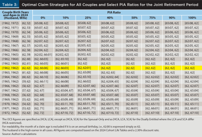
Joint Period

Results for the joint period optimization are shown in Table 3. As the joint period is always shorter than the individual life expectancy of either spouse, earlier claiming at or near 62 by both spouses should be optimal in many cases. Aside from cases with an HCA-restricted SCA, the OCS for couples with spouses close in age differs negligibly from this expected [62, 62] strategy. As the age difference lengthens, the optimal claiming age of the older spouse increases (though never reaching FRA except with the [1972, 1962] couple and in cases of an HCA-restricted SCA). This result is due to the length of the joint period, which is shortest for the same-age couple but longer with increasing age difference (see Table 1). Apparently, as the joint period lengthens, the increase in benefit amount for a few years delay by the currently aged 62 older spouse contributes more to the EMV than would any advantage from the earlier cash flows for claiming at 62. As might be expected, claiming age 62 is optimal for the younger spouse in all couples at nearly all PIA ratios.

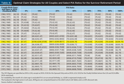
Survivor Period

Results for the survivor period optimization are shown in Table 4. As discussed above, survivor period optimization in this study is the same as full period optimization but with the reference year adjusted to the beginning of the survivor period of each death outcome. Though the resulting EMV figures themselves are different from the straightforward expected present values computed for the full period optimization, the exact same cash flows are included, and as such, large deviations from the full period OCS results should not be expected. In fact, for all couples and PIA ratios, the optimal HCA is equal to, or negligibly different from, that for the full period. Similarly, the optimal LCA is virtually the same as that for the full period in all cases with an older husband. However, with a younger husband, noticeable differences appear and always include a delay by the wife. Whether or not this new method of calculating the EMV for the survivor period is more appropriate remains to be determined but is worth exploring.

Conclusion

This study explored optimal claiming strategies for a series of married couples with a higher-earning husband and lower-earning wife, spanning a range of spousal age differences and covering the full spectrum of spousal PIA ratios. For each couple and PIA ratio, the expected present value of the benefit cash flows was computed for each possible monthly claiming strategy. The claiming strategy with the highest expected present value was selected as the optimal claiming strategy for the given couple and PIA ratio. Optimization was analyzed for three different retirement periods: the full period covering the entire retirement from inception to the death of the widow, the joint period when both spouses are alive, and the survivor period when only the surviving widow is alive.

Perhaps the most obvious conclusion from this study is that optimizing claiming for married couples can be immensely complex. Factors such as the birth cohorts and sexes of the spouses, which determine their age differences and individual survival functions, the ratio of lifetime earnings between the spouses (PIA ratio), the various benefit rules and formulas, and the choice of discount rates and computation methods for the benefit cash flows all interact in the valuation of a claim strategy. In addition, the optimality of the claiming decision is framed here only as maximization of the expected monetary value of lifetime benefits at a single exemplary discount rate, ignoring the possibility that a real-life couple may have entirely different criteria on which to base their decision.

For optimization of the full retirement period, the default strategy is a delayed claim by the high earner, usually to age 70, and an immediate claim by the low earner at or near age 62. The optimality of this default strategy, which both maximizes benefit cash flows during widowhood while also advantageously collecting cash flows during the joint period, holds true in many cases. However, stark deviations from this default strategy appear at various regions across spousal age differences and PIA ratios. Variations in optimal claim strategies over the range of the couples can best be explained by the level of the PIA ratio.

At low PIA ratios where the low-earning wife is entitled to the spousal benefit, the default strategy is generally optimal for couples with an older husband. As the spouses get closer in age, the higher-earning husband must claim earlier than 70 simply to allow the wife to claim her HCA-restricted spousal benefit near enough to 62 to maximize the joint period cash flows. For couples with younger husbands, this trend continues with even earlier claim ages for the husband. Notably, for couples where the husband is only five or more years younger than the wife, his optimal claim age is actually earliest at 62.

At high PIA ratios where the spouses have equal or near equal lifetime earnings, optimality of the default strategy itself no longer applies because neither spouse is a substantially higher earner. In these situations, it is the ability of the older spouse to make the earliest fully delayed claim at age 70 that maximizes the expected present value with the most age 70 benefit payments, received earliest, and thus discounted least. For couples with an older husband at these high PIA ratios, what appears to be the usual default strategy is actually the older husband claiming at age 70 not because he is the higher earner but because he reaches age 70 first, and the younger wife then claiming as soon as possible at 62. For couples with a younger husband, the OCS appears as an inverted default strategy with the older wife claiming at 70 (because she reaches age 70 first) and the younger husband claiming as soon as possible at 62.

Historically, most married couples consisted of an older, higher-earning husband and a younger, lower- or non-earning wife. As Iams (2016) has noted, more than half of married women in 1960 were receiving benefits based solely on their husbands’ earnings. However, projections included in that study indicated that over 80 percent of married women now entering retirement will receive retirement benefits based solely on their own individual earnings. While most are still expected to become survivors switching to widow benefits based on their husband’s record, 30 percent will have a worker benefit from their own record high enough to retain into widowhood. Thus, the results in the present study for couples with high PIA ratios, that is, spouses of near equal earnings histories, should be of increasing interest and importance.

In addition to optimization of the full retirement period, optimal claiming was also explored for the joint and survivor periods, separately. For the joint period optimization, which is the same as the full period optimization above but with survivor period cash flows excluded, early claiming by both spouses at or near age 62 is usually optimal, with any delay always by the older spouse (except for instances of an HCA-restricted SCA). For the survivor period optimization, which is the same computation as the full period optimization but with an adjusted time valuing method, results are very similar to those for the full period, but with a noticeably delayed claim by the older wife in couples with younger husbands. 

Citation

Alleva, Brian J. 2025. “The Social Security Claiming Decision for Married Couples.” Journal of Financial Planning 38 (12): 70–87.

Endnotes

1. The present study assumes that the claiming decision is taking place in isolation from other retirement considerations that married couples often face, such as whether or not a spouse can actually afford to retire at a given age and claim benefits, or conversely, is able and willing to continue working while delaying claiming. Related factors such as the availability of other income sources in retirement to augment Social Security benefits, or the effect of benefits on the couple’s tax situation, are also excluded from consideration.
2. The survival functions used in this study are derived from the cohort life tables prepared by the Office of the Chief Actuary of the Social Security Administration for the Alternative II (intermediate) projections published in the 2024 Trustees’ report (Board of Trustees 2024). These tables provide historical and projected survival probabilities by birth cohort, sex, and single year of age. See www.ssa.gov/OACT/Downloadables/CY/index.html. For complete details on the computation of the survival functions from the life tables, including joint survival functions for a given couple, see Alleva (2016a).
3. Table 1 verifies that the full period expectancy is equal to the sum of the joint and survivor period expectancies for each couple. In addition, for all couples, the full period expectancy is always longer than the life expectancy of either spouse as the likelihood of at least one spouse alive is less restrictive than the likelihood of any individual spouse alive. The reverse is true for the joint period expectancy, which is always less than the life expectancy of either spouse, as the likelihood of both spouses alive is more restrictive than the likelihood of any individual spouse alive.
4. For more information on the PIA, see www.ssa.gov/OACT/COLA/piaformula.html. For more information on the FRA (also known as the normal retirement age), see www.ssa.gov/OACT/ProgData/nra.html.
5. For more information about working during retirement, see www.ssa.gov/benefits/retirement/planner/whileworking.html and www.ssa.gov/pubs/EN-05-10069.pdf.
6. For more information on worker and spousal benefit claiming rules, see Alleva (2017).
7. The term “widow” is applied here to both surviving wives and surviving husbands.
8. For cohorts born earlier than 1962, the survivor FRA, generally a few months younger than the actual FRA, is used for the widow benefit calculation. For cohorts born 1962 and later, and thus for all cohorts referenced in this study, the FRA and the survivor FRA are both 67, and so the distinction is no longer necessary.
9. For general information about widow benefit claiming rules and formulas, see:
   www.ssa.gov/survivor, www.ssa.gov/OP_Home/handbook/handbook.07/handbook-0724.html, and www.ssa.gov/OP_Home/handbook/handbook.04/handbook-0401.html.
   For documentation of the calculation of the full widow benefit (i.e., b), see: www.ssa.gov/OP_Home/handbook/handbook.04/handbook-0407.html and www.ssa.gov/OP_Home/handbook/handbook.07/handbook-0720.html.
   For more information regarding switching between worker and widow benefits, see: www.ssa.gov/survivor and www.ssa.gov/OP_Home/handbook/handbook.04/handbook-0409.html.
   For excellent presentations of the widow benefit claiming rules and their application to various situations, see Reichenstein and Meyer (2016) and Davies and Li (2022).
10. See Alleva (2017) for a discussion on the determination of possible claim strategies.
11. Shuart et al. (2010) explored delayed widow benefit claiming in greater detail.
12. The ultimate real rate of 2.3 percent is used for the Alternative II (intermediate) assumption set. See section V.B.7 on page 116 in Board of Trustees (2024).
13. Alleva (2015) similarly analyzed different target periods of retirement for claiming optimization for individuals.
14. Note that survival to age 62 is an important requirement for computing the EMV of a claim strategy. Considering that 62 is the earliest age at which worker benefits can be claimed, if the death of either spouse were to occur before age 62, then no claim age could be executed, EMVs for all claim ages for that spouse would be zero, and the question of which claim age is maximizing would be moot.
15. The “reality” of the survivor period financial experience is the rationale for this method. As an example, for a given claim strategy, a five-year widowhood beginning at age 72 should be considered a very different situation than a five-year widowhood beginning at age 95. If all joint period cash flows are invested at the selected discount rate (that is, future-valued) for consumption only during the survivor period, the 95-year-old widow would be in a vastly better financial position than her 72-year-old counterpart, due simply to the greater number of benefit payments invested for a longer period of time. Though such scenarios might require extraordinary investing discipline, if optimization of the survivor period is the chosen objective of the claiming strategy, then the assumption is valid, and the actual financial experiences implied by these two death outcomes should be weighed in the OCS computation accordingly.

References

Alleva, Brian J. 2015. “Minimizing the Risk of Opportunity Loss in the Social Security Claiming Decision.” Journal of Retirement 3 (1): 67–86.

Alleva, Brian J. 2016a. “The Longevity Visualizer: An Analytic Tool for Exploring the Cohort Mortality Data Produced by the Office of the Chief Actuary.” Social Security Administration Research and Statistics Note 2016-02. www.socialsecurity.gov/policy/docs/rsnotes/rsn2016-02.html.

Alleva, Brian J. 2016b. “Discount Rate Specification and the Social Security Claiming Decision.” Social Security Bulletin 76 (2): 1–15. www.ssa.gov/policy/docs/ssb/v76n2/v76n2p1.html.

Alleva, Brian J. 2017. “Social Security Retirement Benefit Claiming-Age Combinations Available to Married Couples.” Social Security Administration Research and Statistics Note 2017-01. https://www.ssa.gov/policy/docs/rsnotes/rsn2017-01.html.

Board of Trustees, Federal Old-Age and Survivors Insurance and Federal Disability Insurance Trust Funds. 2024. The 2024 Annual Report of the Board of Trustees of the Federal Old-Age and Survivors Insurance and Federal Disability Insurance Trust Funds. Washington, DC: Government Printing Office. www.ssa.gov/OACT/TR/2024/tr2024.pdf.

Davies, Paul S., and Zhe Li. 2022. “Social Security: The Widow(er)’s Limit Provision.” Congressional Research Service. https://crsreports.congress.gov/product/pdf/IF/IF12091.

Iams, Howard M. 2016. “Married Women’s Projected Retirement Benefits: An Update.” Social Security Bulletin 76 (2): 17–24. www.ssa.gov/policy/docs/ssb/v76n2/v76n2p17.html

Meyer, William, and William Reichenstein. 2010. “Social Security: When Should You Start Benefits and How to Minimize Longevity Risk?” Journal of Financial Planning 23 (3): 52–63.

Munnell, Alicia H., and Mauricio Soto. 2007. “When Should Women Claim Social Security Benefits?” Journal of Financial Planning 20 (6): 58–65.

Reichenstein, William, and William Meyer. 2016. “Social Security Claiming Strategies for Widows and Widowers.” Journal of Retirement 3 (4): 77–86.

Sass, Steven A., Wei Sun, and Anthony Webb. 2007. “Why Do Married Men Claim Social Security Benefits So Early? Ignorance or Caddishness?” Center for Retirement Research at Boston College Working Paper 2007–17.

Shoven, John B., and Sita N. Slavov. 2014a. “Recent Changes in the Gains from Delaying Social Security.” Journal of Financial Planning 27 (3): 32–41.

Shoven, John B., and Sita N. Slavov. 2014b. “Does it Pay to Delay Social Security?” Journal of Pension Economics and Finance 13 (2): 121–144.

Shuart, Amy N., David A. Weaver, and Kevin Whitman. 2010. “Widowed Before Retirement: Social Security Benefit Claiming Strategies.” Journal of Financial Planning 23 (4): 45–53.

Sun, Wei, and Anthony Webb. 2011. “Valuing the Longevity Insurance Acquired by Delayed Claiming of Social Security.” Journal of Risk and Insurance 78 (4): 907–929.