Journal of Financial Planning: April 2016
Andrew Miller, CFA, CFP®, is chief investment officer at Miller Financial Management LLC, where he is primarily responsible for investment and financial planning research, asset allocation, and integrating clients’ financial plans with their investment portfolios. His research interest is in using academic investment research to create investment portfolios that improve the withdrawal rates and financial outcomes for clients.
Acknowledgement: The author thanks Chris Miller, CPA/PFS, CFP®, and Wesley Gray, Ph.D., for their invaluable comments, patience, and insights.
Executive Summary
- Using historical simulation, a 4 percent initial withdrawal rate from a 50/50 stock/bond portfolio with a 30-year time horizon has a failure rate between 0 and 5 percent, depending on the bond index used.
- Recent research shows that if one adjusts return assumptions using valuation and/or current bond yields, the failure rate of an initial 4 percent withdrawal rate increases dramatically to between 18 and 57 percent, depending on the assumptions.
- Because low bond yields are the primary cause of the increase in failure rates of an initial 4 percent withdrawal rate, it is possible to create an investment portfolio with the same stock market beta of a 50/50 stock/bond portfolio, but with a smaller allocation to bonds.
- A minimum variance stock portfolio was used in a portfolio with intermediate-term bonds to create a portfolio with a 0.5 market beta. The new portfolio has a marked increase in a “safe” initial withdrawal rate using historical data.
- Using a Monte Carlo engine and current yield information, the new portfolio has a lower failure rate at an initial 4 percent withdrawal rate and/or it supports an increased withdrawal rate at a given acceptable failure rate.
Determining an appropriate withdrawal rate from their investment portfolios is one of the biggest investment or financial planning decisions retirees will make. Prior research indicates that a portfolio of 50 percent stocks and 50 percent bonds is capable of supporting an initial withdrawal rate of 4 percent (with the dollar amount subsequently adjusted for inflation). Bengen (1994) showed that a 4 percent initial withdrawal rate failed in 0 percent of historical simulations. In addition, using Monte Carlo simulations, with capital market expectations equal to the historical averages, the 4 percent initial withdrawal rate failed in only 6 percent of the simulations.
However, for a 4 percent initial withdrawal rate to continue to be successful 95 percent or more of the time, then one must also assume that future stock and bond returns will be much like (or better than) the past, with arithmetic average rates of return of 8.7 percent above inflation for stocks and 2.1 percent above inflation for bonds. Unfortunately, current retirees are likely to earn rates of return far below those historical figures. One cause for the likely decrease in future returns are the depressed real yields on bonds. As of June 30, 2015 the real yield on five-year Treasury inflation-protected securities (TIPS) stood at 0.02 percent, and the real yield on 30-year TIPS stood at 1.1 percent.
Finke, Pfau, and Blanchett (2013) showed that “safe” withdrawal rates changed dramatically when stock and bond returns were adjusted for current valuations. For example, the authors investigated the following scenario: (1) decrease the arithmetic returns of stocks and bonds by 2.1 percent per year to make the real return on bonds approximately 0 percent; and (2) decrease the return on stocks to maintain the historical return premium of stocks over bonds. Using these assumptions, an initial 4 percent withdrawal rate failed in approximately 33 percent of simulations compared to only 6 percent of simulations using historical average returns. These results demonstrated that given current real bond yields, an initial 4 percent withdrawal rate can no longer be considered safe.
One way to increase the safe withdrawal rate of a portfolio is to decrease the allocation to bonds and increase the allocation to stocks. Unfortunately, increasing the allocation to stocks dramatically changes the risk profile of the portfolio by increasing the standard deviation of returns and increasing the maximum drawdown. Increasing the risk profile may make the resulting portfolio inappropriate for an investor by making the portfolio more volatile than his or her risk preference, or it may cause the investor to make the portfolio less aggressive in the middle (or end) of a drawdown, thereby eliminating the benefit of an increased “safe” withdrawal rate that a risker asset allocation may provide.
This study proposed a solution to this conundrum—to use a low-volatility stock portfolio as the primary asset class in the portfolio. A portfolio constructed primarily of low-volatility stocks allows an investor to decrease the allocation to lower-yielding bonds while maintaining a similar risk profile to a traditional 50/50 stock/bond portfolio. The disadvantage of this solution is an increase in benchmark tracking risk. In addition, it is not a market cap weighted portfolio, so by definition, it isn’t a viable alternative for all investors.
Low-Volatility Stocks
Black, Jensen, and Scholes (1972) conducted breakthrough research on the low volatility effect. The authors showed that stock returns were not proportional to their market betas (i.e., low-volatility stocks have similar returns as high-volatility stocks). In addition, Black (1972) found that some investors were unable or unwilling to borrow funds to purchase the cohort of stocks that were less volatile. Therefore, those investors over-weighed volatile stocks, thereby increasing their prices and lowering future returns, and those same leverage constrained investors under-weighed low-volatility stocks, thereby depressing their prices and raising their future returns. More recent work on the low volatility anomaly by Haugen and Baker (2012) and Frazzini and Pedersen (2014) confirmed Black, Jensen, and Scholes’ original findings.
Frazzini and Pedersen (2014) and Black (1972) cited leverage aversion as the source of the low volatility anomaly. In addition, the leverage aversion theory in Frazzini and Pedersen (2014) was able to explain the low volatility anomaly in other asset classes and investment styles. Therefore, this study used the theory of leverage aversion/constraints to create a portfolio composed of low-volatility stocks and bonds that had similar risk characteristics (standard deviation and beta to the stock market) as a traditional 50/50 stock/bond portfolio, but the low-volatility stock portfolio was shown to be able to support an increase in “safe” withdrawal rates.
Practically speaking, many investors have constraints on their ability to use leverage. An obvious example is the inability to use margin inside of an IRA. This constraint on leverage would likely affect many different types of investors including most individual investors (i.e., the type of investor who would be following a 4 percent initial withdrawal rate rule).
Interestingly, the 4 percent initial withdrawal rate cited in Bengen (1994) was calculated using a portfolio with a 50 percent allocation to intermediate-term (i.e., five-year) government bonds. Even though most individual investors have leverage constraints, they do have the ability to decrease their allocation to intermediate-term bonds, which would have an economically similar impact of using leverage.
When viewed in this light, most investors who contemplate a 4 percent initial withdrawal rule do have an ability to indirectly leverage their portfolio by decreasing their allocation to intermediate-term bonds and purchasing low-volatility stocks. This portfolio construct allows an investor to capture the additional return from low-volatility stocks while maintaining a similar risk profile as a traditional market cap weighted 50 percent stock, 50 percent bond portfolio.
Safe Withdrawal Rates
Most withdrawal rate studies can be grouped into two main categories: historical simulation and Monte Carlo simulation.
Historical simulation is the use of rolling 30-year asset class return series (typically using Ibbotson Associates’ Stocks, Bonds, Bills, and Inflation for U.S. asset classes since 1926) to determine an initial withdrawal rate for each 30-year rolling period. The smallest initial withdrawal rate of all the 30-year rolling periods is used as the maximum sustainable withdrawal rate, or what Bengen eventually called “SAFEMAX.” Some of the most popular studies to use historical simulation are Bengen (1994) and Cooley, Hubbard, and Walz (1998).
Monte Carlo simulations have several advantages over historical simulation. The first is that historical simulation tends to overweigh the importance of returns in the middle years of the data series, as they appear most often in the rolling 30-year periods (for example, 1926 only appears in one rolling 30-year period, but 1956 appears in 31 rolling 30-year periods). The second advantage of Monte Carlo simulation is that it allows for a potentially unlimited number of trial runs where historical simulation is limited.
Monte Carlo simulation tends to come in two varieties. One is bootstrapping, which involves randomly selected historical data used to artificially create rolling 30-year returns. The second uses a random number generator and a probability distribution, where the parameters of the distribution are determined by the user to create rolling 30-year returns. Most studies tend to use historical inputs for returns, standard deviation, and correlations to define the probability distributions.
However, Finke, Pfau, and Blanchett (2013) used Monte Carlo simulation and adjusted the average returns of bonds to reflect lower current real yields. They adjusted stock returns downward by the same amount to keep the same return premium for stocks over bonds. They recalculated SAFEMAX for various asset allocations and arrived at substantially lower SAFEMAXs than if one were to use historical simulation.
This study followed a hybrid approach, using all three approaches: historical simulation, Monte Carlo simulation with probability distributions based off of historical inputs, and Monte Carlo simulation with probability distributions adjusted to reflect similar inputs as Finke, Pfau, and Blanchett (2013).
Data
Ibbotson Associates’ time series data for Stocks, Bonds, Bills, and Inflation was used, specifically, the IA SBBI U.S. Large Cap TR, the IA SBBI Intermediate-Term Government TR, the IA SBBI U.S. 30-Day Bills TR, and the IA SBBI Inflation time series.
The low volatility time series was constructed by using the regression analysis for the U.S. minimum variance (PCA) portfolio in Chow, Hsu, Kuo, and Li (2014).
The data inputs for the statistical recreation were from the AQR data library (www.aqr.com/library) for the Mkt-RF factor, SMB (size), HML (value), and BAB (betting against beta) factor. The Kenneth R. French data library (mba.tuck.dartmouth.edu/pages/faculty/ken.french/data_library.html) was used for the WML (momentum) factor.
The DUR (bond duration) factor was constructed as the return of the IA SBBI Long-Term Government TR less the IA SBBI U.S. 30-Day Bills TR. The risk-free rate was set to IA SBBI U.S. 30-Day Bills TR.
For the statistical recreation, because the regression intercept in Chow, Hsu, Kuo, and Li (2014) was not statistically significant, 0 percent was used, making the statistical recreation slightly conservative.
The factor returns noted previously closely matched the factor series in Chow, Hsu, Kuo, and Li (2014) Appendix 1, with the exception of the BAB factor, which showed a factor premium of 4.82 percent and a factor Sharpe ratio of 0.41. This was not the same as the BAB factor in the AQR library, or in the related work by Frazzini and Pedersen (2014), which showed a factor premium of approximately 11.1 percent and a factor Sharpe ratio of approximately 0.95.
In order to recreate results similar to Chow, Hsu, Kuo, and Li (2014), the BAB factor from the AQR library was multiplied by a constant 41 percent so that the BAB factor premiums were equal (even though multiplying by a constant of 41 percent still made the Sharpe ratio 0.95).
Following this procedure, for the period of January 1, 1967 through December 31, 2012 the differences in return (11.36 percent) and standard deviation (10.52 percent) of the statistical recreation, and the return (11.38 percent) and risk (11.52 percent) shown in Chow, Hsu, Kuo, and Li (2014) were not particularly notable.
The statistical recreation of a minimum volatility portfolio was then extended back to 1931 (the beginning of the BAB factor returns) using the same factor loadings and 41 percent constant of BAB as was shown in Chow, Hsu, Kuo, and Li (2014).
Methodology
The historical simulation started retirement at the first year of available data (1931–2013), and an initial withdrawal was made equal to the specified initial withdrawal rate times the beginning portfolio balance. The remaining balance then grew or shrank according to the asset return for that year. At the end of the year, the remaining portfolio was rebalanced back to the target asset allocation. Taxes, fees, and trading costs were ignored to remain consistent with prior studies.
The next year, the withdrawal amount was adjusted upward or downward by the previous year’s inflation rate, and the portfolio grew or shrank according to the asset return for that year. The withdrawal amount was only adjusted by inflation so that the withdrawal rate would be a different percentage of the portfolio every year (in other words, the withdrawal amount was only changed by inflation, not asset returns).
An iterative operation was used for the first 30-year period that set the ending wealth equal to $0 by changing the initial withdrawal percentage. The initial withdrawal percentage that set the ending wealth equal to $0 was called the maximum withdrawal rate (MWR). The MWR was noted for each rolling 30-year period until the end of the data. The smallest MWR from all rolling 30-year periods was considered the SAFEMAX.
For the Monte Carlo simulation based on historical data, a lognormal distribution with the data inputs shown in Table 1 was used.
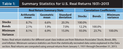
Following the same logic as Finke, Pfau, and Blanchett (2013), and in consideration of five-year TIPS bonds trading at a real yield of 0.02 percent as of June 30, 2015, the geometric mean return of bonds was reduced from 1.9 percent to 0 percent. In addition, the geometric mean return of stocks and a minimum variance portfolio of stocks were reduced by the same 1.9 percent to keep a consistent risk premium of stocks over bonds.
The second set of assumptions for the Monte Carlo simulation are shown in Table 2.
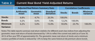
The portfolio that used a portfolio construct of minimum variance stocks and a reduced allocation to bonds had a 70 percent allocation to minimum variance stocks and a 30 percent allocation to intermediate-term bonds. The weights for this portfolio were derived using two different methods.
First, the minimum variance stock and intermediate-term bond portfolio couldn’t have a materially greater standard deviation than the 50 percent market cap weighted stock and 50 percent intermediate-term bond portfolio, because it was important to eliminate the chance that SAFEMAX differs due to differences in standard deviation between the two portfolios. Making some general assumptions that (1) a minimum variance stock portfolio was three quarters as volatile as a market cap weighted stock portfolio; (2) the correlation between market cap weighted stocks and intermediate-term bonds was 0 percent; and (3) the correlation between a minimum variance stock portfolio and intermediate-term bonds was 0 percent, then a portfolio of 70 percent minimum variance stocks and 30 percent intermediate-term bonds would have the same standard deviation as a portfolio of 50 percent market cap weighted stocks and 50 percent intermediate-term bonds.
Using these weights, the historical standard deviation of a 70 percent minimum variance stock portfolio and 30 percent intermediate-term bond portfolio was 10.4 percent per year. The historical standard deviation of a 50 percent market cap weighted stock and 50 percent intermediate-term bond portfolio was 10.3 percent per year.
Second, the minimum variance stock and intermediate-term bond portfolio couldn’t have a materially different factor loading to the MKT risk factor than a 50 percent market cap weighted stock and 50 percent intermediate-term bond portfolio. Making a general assumption that a minimum variance portfolio would have a factor loading of 0.7 to the MKT risk factor meant that a portfolio of 70 percent minimum variance stocks and 30 percent intermediate-term bonds would have a total factor loading of 0.49 to the MKT risk factor, versus a factor loading of 0.5 to the MKT risk factor for a portfolio of 50 percent market cap weighted stocks and 50 percent intermediate-term bonds.
Using historical return series, a portfolio of 70 percent minimum variance stocks and 30 percent intermediate-term bonds had a factor loading of 0.47 to the MKT risk factor. Therefore, any difference in SAFEMAX or any other withdrawal rate measures could be directly attributable to differences in the construction of the portfolio, and not due to different levels of standard deviation or to different factor loadings to the MKT risk factor. Conversely, any differences were attributable to decreasing reliance on bond returns and more reliance on the low volatility anomaly.
Results
The historical simulation showed that the SAFEMAX for a portfolio of 70 percent minimum volatility stocks and 30 percent intermediate-term government bonds was 4.7 percent, and the 30-year rolling period associated with the SAFEMAX started in 1937. This result compared favorably with a 50 percent market cap weighted stock and 50 percent intermediate-term government bond portfolio that Bengen (1994) showed had a SAFEMAX of approximately 4 percent. The 30-year rolling period associated with the SAFEMAX in Bengen (1994) started in 1966.
Table 3 shows the failure rate for an initial 4 percent withdrawal rate for the two different asset allocations studied in this paper and for both sets of assumptions used for the Monte Carlo analysis. Failure rates were highly sensitive to reductions in return assumptions. For example, when you decreased the geometric return of all assets by 1.9 percent, the failure rate of an initial 4 percent withdrawal rate increased four-fold from 8 percent to 32 percent.
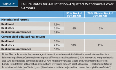
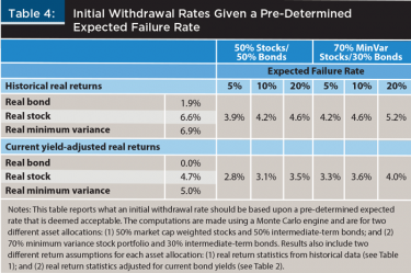
Table 4 shows a “safe” initial withdrawal rate for the two asset allocations studied in this paper for pre-determined acceptable failure rates of 5, 10, and 20 percent, and for different asset return assumptions.
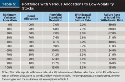
To test the robustness of the improvement in withdrawal rates from using low-volatility (minimum variance) stocks in a portfolio, multiple portfolios with varying allocations of low-volatility stocks and bonds were created. The portfolios ranged from 0 percent low-volatility stocks and 100 percent bonds to 100 percent low-volatility stocks and 0 percent bonds in 10 percent increments.
Table 5 shows the resulting portfolio standard deviation, using the assumptions in Table 2 for each allocation of low-volatility stocks and bonds.
As a baseline comparison, and using the assumptions in Table 2, a portfolio of market cap weighted stocks and bonds was created so that the market cap weighted stock and bond portfolio had the same standard deviation as a comparable portfolio of low-volatility stocks and bonds. These results are shown in Table 6. These baseline comparison portfolios were created so that any differences in withdrawal rates between a portfolio of low-volatility stocks and bonds and a portfolio of market cap weighted stocks and bonds were due to portfolio construction and not differences in portfolio risk levels.
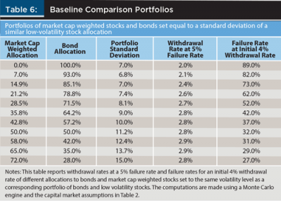
A Monte Carlo analysis was run using the assumptions in Table 2 and the portfolio allocations in Tables 5 and 6. The initial withdrawal rate that resulted in a 5 percent failure was noted for each of the 20 allocations in Tables 5 and 6 respectively. The failure rate of an initial 4 percent withdrawal was also noted in Tables 5 and 6.
A comparison of Tables 5 and 6 demonstrates that every portfolio that contained low-volatility stocks had a higher withdrawal rate at a 5 percent failure rate than a portfolio with the same volatility level, but that was constructed using market cap weighted stocks and bonds.
A comparison of Tables 5 and 6 also shows that every portfolio that contained low-volatility stocks had a lower failure rate, given an initial 4 percent withdrawal, than a portfolio comprised of market cap weighted stocks and bonds with the same volatility level.
Conclusion
Determining a safe initial withdrawal rate from a portfolio at the start of retirement may be one of the most important decisions an investor makes. Most research regarding initial withdrawal rates implicitly or explicitly used historical average rates of return for asset classes in determining the safe initial withdrawal rate. However, recent research has shown, and this paper supports, the notion that lowering return assumptions for asset classes can have a substantial impact on failure rates of an initial 4 percent withdrawal rate. In particular, lowering the assumed rate of return for bonds and stocks by 1.9 percent can cause a fourfold increase in the failure rate of a 4 percent initial withdrawal from a 50/50 stock/bond portfolio.
Investors don’t have to passively accept either higher failure rates or lower withdrawal rates. By leveraging the benefits of the low volatility anomaly, an investor can create a portfolio with the same standard deviation and market beta as a traditional 50 percent market cap stock and 50 percent intermediate-term bond portfolio, but with either an increase in an initial withdrawal rate or a decrease in failure rate given an initial withdrawal rate.
References
Bengen, William P. 1994. “Determining Withdrawal Rates Using Historical Data.” Journal of Financial Planning 7 (4): 171–180.
Black, Fisher, 1972. “Capital Market Equilibrium with Restricted Borrowing.” Journal of Business 45 (3): 444–455.
Black, Fisher, Michael C. Jensen, and Myron Scholes, 1972. “The Capital Asset Pricing Model: Some Empirical Tests.” In Studies in the Theory of Capital Markets, edited by M. C. Jensen. New York: Praeger, 79–121.
Chow, Tzee-Man, Jason C. Hsu, Li-Lan Kuo, and Feifei Li. 2014. “A Study of Low-Volatility Portfolio Construction Methods.” The Journal of Portfolio Management 40 (4): 89–105.
Cooley, Philip L., Carl M. Hubbard, and Daniel T. Walz. 1998. “Retirement Savings: Choosing a Withdrawal Rate that Is Sustainable.” Journal of the American Association of Individual Investors 20 (2): 16–21.
Finke, Michael, Wade D. Pfau, and David M. Blanchett. 2013. “The 4 Percent Rule Is Not Safe in a Low-Yield World.” Journal of Financial Planning 26 (6): 46–55.
Frazzini, Andrea, and Lasse H. Pedersen. 2014. “Betting Against Beta.” Journal of Financial Economics 111 (1): 1–25.
Haugen, Robert A., and Nardin L. Baker. 2012. “Low Risk Stocks Outperform within All Observable Markets of the World.” Haugen Custom Financial Systems and Guggenheim Investments working paper.
Citation
Miller, Andrew. 2016. “Improving Withdrawal Rates in a Low-Yield World.” Journal of Financial Planning 29 (4): 52–58.